A dive into computer vision via Convolutional Neural Networks and how the Winograd Convolution is implemented. CNNs are one of the most elegant examples of inductive bias in deep learning — the assumption that spatial locality matters, baked directly into the architecture.
What This Post Covers
- Convolution as a Linear Operation — The convolution theorem, Toeplitz matrices, and why convolution is really just structured matrix multiplication
- CNN Architectures — From LeNet to ResNet, how the field evolved its understanding of depth and skip connections
- The Winograd Transform — A lesser-known optimization that reduces the number of multiplications in convolution by trading them for additions, yielding significant speedups for small filter sizes
- Implementation Details — Memory layout (NCHW vs NHWC), im2col tricks, and why GPU implementations don’t always match the textbook
Why Winograd?
Standard convolution requires \(O(m \cdot k^2)\) multiplications per output element. Winograd’s minimal filtering algorithm reduces this to roughly \(O(m)\) multiplications at the cost of more additions and a larger transformed tile. For 3x3 filters — the most common in modern architectures — this translates to real-world speedups of 2-4x.
What Is Convolution?
What are some ways to combine two functions $f$ and $g$ to get a third function $h$? We could add them ($h = f + g$), multiply them ($h = f \cdot g$), or compose them ($h = f \circ g$). There is another way — less commonly encountered outside of signal processing and probability — called convolution.
Definition. The convolution of $f$ and $g$ is defined as
\[(f * g)(t) \stackrel{\text{def}}{=} \int_{-\infty}^{\infty} f(\tau) \, g(t - \tau) \, d\tau.\]The idea: flip $g$, slide it across $f$, and at each position $t$, compute the integral of their overlap. Convolution measures how much one function “agrees” with a shifted, reversed copy of another — a weighted average where the weights come from the kernel function itself.
Convolutions appear throughout mathematics: in signal processing (filtering), probability (the PDF of a sum of independent random variables is the convolution of their individual PDFs), differential equations, and polynomial multiplication. We will focus on their application to images.
Discrete 2D Convolution
For images, we replace the integral with a sum and work in two dimensions. Given an image $I$ and a small matrix $K$ called a kernel (or filter), the discrete 2D convolution is
\[(I * K)[i, j] = \sum_{m} \sum_{n} I[i + m, \, j + n] \cdot K[m, n].\]The kernel slides across the image. At each position $[i, j]$, we lay the kernel on top of the image, compute the elementwise product of the overlapping values, and sum the results. The region of the image that the kernel covers at a given position is called the receptive field.
A 3x3 kernel slides over the input image. At each position, the output is the sum of elementwise products between the kernel and the receptive field (dashed region).
Convolution is a local operation — each output pixel depends only on a small neighborhood of the input. This is the inductive bias of CNNs: spatial locality matters. Nearby pixels are more relevant to each other than distant ones.
Kernels in the Wild
The choice of kernel determines what the convolution detects. Different kernels extract different features from an image, and understanding them builds intuition for why learned kernels are so powerful.
Gaussian Blur
The simplest useful kernel is the Gaussian blur. To blur an image, we want each output pixel to be a weighted average of its neighbors, with closer neighbors receiving more weight. A natural choice is to sample the kernel values from a Gaussian distribution.
A 5x5 Gaussian kernel. The center pixel gets the most weight (41/273); weights taper symmetrically with distance.
The center pixel receives the most weight, and influence tapers with distance. The normalization factor $1/273$ ensures the weights sum to one, preserving overall brightness. For pixels near the edges of the image, we pad the boundary — typically by repeating edge values or filling with zeros — so the kernel always has a full receptive field.
Gabor Filters
A more interesting class of kernels detects edges. A Gabor filter is a sinusoidal plane wave modulated by a Gaussian envelope. Each Gabor filter is tuned to a specific orientation and frequency, making it sensitive to edges at a particular angle.
Gabor filters are special: they appear almost universally in the first layer of trained vision models. Any particular Gabor filter detects changes in a specific direction. By composing several Gabor filters of varying orientations and phases, we can build detectors for increasingly complex structures — stripes, hatches, lines, curves, corners, and even circles. Linear combinations of Gabor filters covering 180 degrees (not 360, because a filter is its own negative reciprocal — variance from left-to-right equals variance from right-to-left) provide powerful edge detection.
Color Contrast Filters
Another primitive kernel type is the color contrast filter. Rather than detecting luminance edges, these kernels respond when one side of the receptive field is the opposite color of the other side. A spider on a leaf, a red car against a blue sky — color boundaries carry information that luminance edges miss.
The Limitation of Hand-Designed Kernels
We could keep going — designing kernels for textures, corners, specific shapes. But hand-coding every kernel we might need does not scale. Images are extraordinarily complex, and we do not give our visual cortexes enough credit. As Rich Sutton observed in his influential essay:
The history of computer vision is a case study in the Bitter Lesson: hand-designed features (SIFT, HOG, Gabor banks) were systematically replaced by learned features. General-purpose methods that leverage computation ultimately win over hand-engineered approaches. The question became not which kernels to use, but how to learn them.
Why don’t we just let a neural network learn the kernels instead? That is exactly what convolutional neural networks do.
Convolution as a Linear Operation
Before we look at CNN architectures, we need to understand a key mathematical fact: convolution is linear. Specifically, it is equivalent to multiplication by a structured matrix. This connection unlocks the entire toolkit of linear algebra for analyzing and optimizing convolutions.
Definition. A Toeplitz matrix is a matrix in which each descending diagonal from left to right is constant:
\[T = \begin{bmatrix} t_0 & t_{-1} & t_{-2} & \cdots \\ t_1 & t_0 & t_{-1} & \cdots \\ t_2 & t_1 & t_0 & \cdots \\ \vdots & & & \ddots \end{bmatrix}\]A Toeplitz matrix is entirely determined by its first row and first column — at most $2n - 1$ values instead of $n^2$.
Convolution as Matrix Multiplication
Consider a 1D convolution of a signal $\mathbf{x} = [x_0, x_1, x_2, x_3]$ with a kernel $\mathbf{k} = [k_0, k_1, k_2]$. Writing out the outputs:
\[\begin{aligned} y_0 &= k_0 x_0 + k_1 x_1 + k_2 x_2 \\ y_1 &= k_0 x_1 + k_1 x_2 + k_2 x_3 \end{aligned}\]This is exactly $\mathbf{y} = T\mathbf{x}$, where $T$ is the Toeplitz matrix constructed from $\mathbf{k}$:
\[T = \begin{bmatrix} k_0 & k_1 & k_2 & 0 \\ 0 & k_0 & k_1 & k_2 \end{bmatrix}\]Each row of the Toeplitz matrix is the kernel shifted by one position. Convolution is structured matrix multiplication.
For 2D images, the structure generalizes to a doubly-block Toeplitz matrix — a block matrix where each block is itself Toeplitz. The details are messier but the principle is the same: 2D convolution is a matrix-vector product with special structure.
The Convolution Theorem
The connection to linear algebra gives us a powerful tool for fast computation.
Theorem (Convolution Theorem). Convolution in the spatial domain corresponds to pointwise multiplication in the frequency domain:
\[\mathcal{F}\\{f * g\\} = \mathcal{F}\\{f\\} \cdot \mathcal{F}\\{g\\}\]where $\mathcal{F}$ denotes the Fourier transform.
This means we can compute a convolution by: (1) FFT both the input and kernel, (2) multiply pointwise, (3) inverse FFT the result. For large kernels, this reduces $O(n \cdot k)$ spatial convolution to $O(n \log n)$ — a significant speedup.
| Method | Multiplications | Best For |
|---|---|---|
| Direct (spatial) | $O(n \cdot k)$ | Small kernels |
| FFT-based | $O(n \log n)$ | Large kernels ($k \gg 3$) |
| Winograd | $\approx O(n)$ mults | Small kernels (3x3) |
But modern CNN architectures overwhelmingly use 3x3 kernels — a design choice we will trace in the next section. For kernels this small, the FFT overhead (transforms, complex arithmetic, memory) is not worth it. This is where the Winograd transform enters the picture.
CNN Architectures
The idea of letting neural networks learn their own kernels — rather than hand-designing them — is the core insight behind convolutional neural networks. Instead of specifying what each filter should detect, we initialize kernels randomly and let gradient descent find filters that minimize a loss function. This is a powerful instance of what Andrej Karpathy calls Software 2.0: instead of writing explicit programs, we specify an objective and let optimization write the program for us.
A Brief Architectural History
LeNet-5 (1998) was the original CNN, designed by Yann LeCun for handwritten digit recognition. Two convolutional layers, subsampling (pooling), and fully connected layers. It worked, but the compute and data available at the time limited its reach.
AlexNet (2012) was the ImageNet moment — the first time a deep CNN decisively won a large-scale image classification competition. Deeper and wider than LeNet, it used ReLU activations, dropout, and crucially, GPU training. AlexNet proved that learned features could surpass decades of hand-engineered feature extractors (SIFT, HOG, Haar cascades) given sufficient data and compute.
VGGNet (2014) contributed a key architectural insight: replace large kernels with stacks of small ones. Two stacked 3x3 convolutions have the same receptive field as a single 5x5 convolution, but with fewer parameters and an extra nonlinearity. Three stacked 3x3 layers match a 7x7 receptive field. This made 3x3 the standard kernel size — which directly motivates the Winograd optimization later.
ResNet (2015) solved the degradation problem. Counterintuitively, deeper networks were performing worse than shallower ones — not from overfitting, but because stacking many nonlinear layers makes it hard to learn the identity function. The fix: skip connections.
Definition. A residual block computes
\[\mathbf{y} = \mathcal{F}(\mathbf{x}, \\{W_i\\}) + \mathbf{x}\]where $\mathcal{F}$ is the residual mapping to be learned. The network only needs to learn the difference from identity, which is easier to optimize. If a layer should act as identity, the residual $\mathcal{F}$ can simply converge to zero.
What Networks Actually Learn
Once we train a CNN, its kernels are just matrices of learned weights — not directly interpretable by looking at the numbers. But through feature visualization — optimizing a random noise image to maximally activate specific neurons — we can see what each layer has learned to detect.
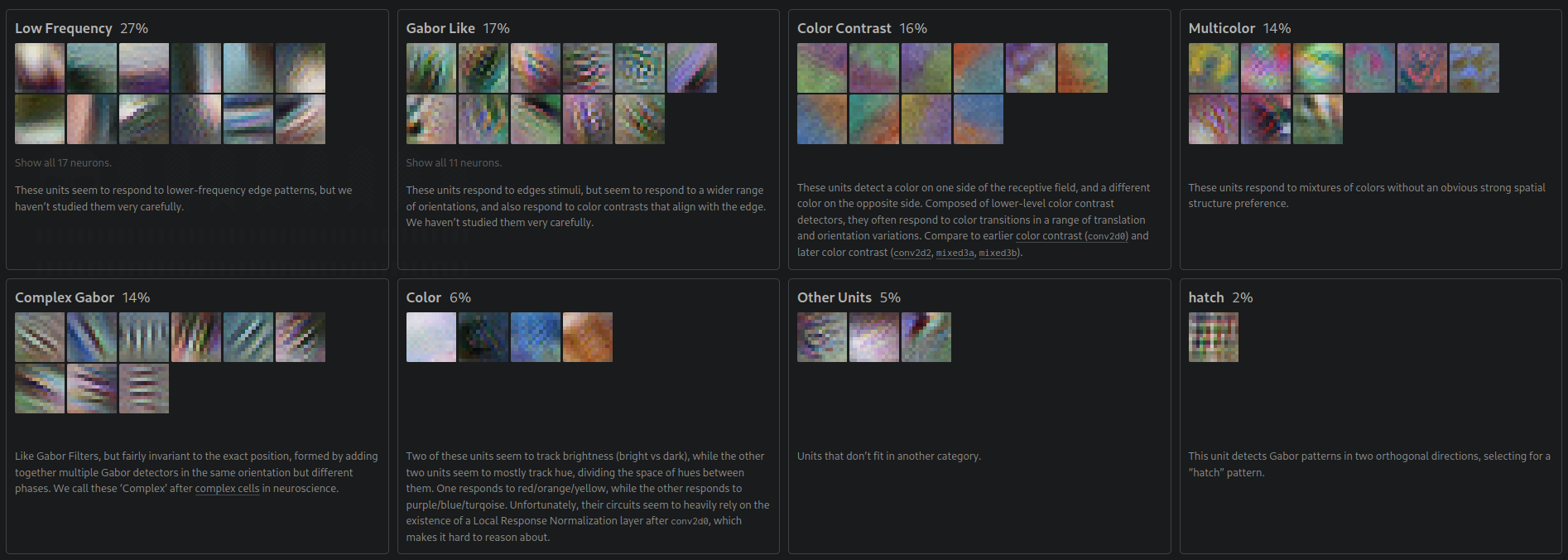
The following visualizations are from Google’s InceptionV1 model, produced by interpretability researchers studying what each convolutional layer encodes.
In the second layer, we see low-frequency patterns, Gabor-like edge detectors, and color contrast neurons — the network independently rediscovered the same primitives that signal processing engineers designed by hand:
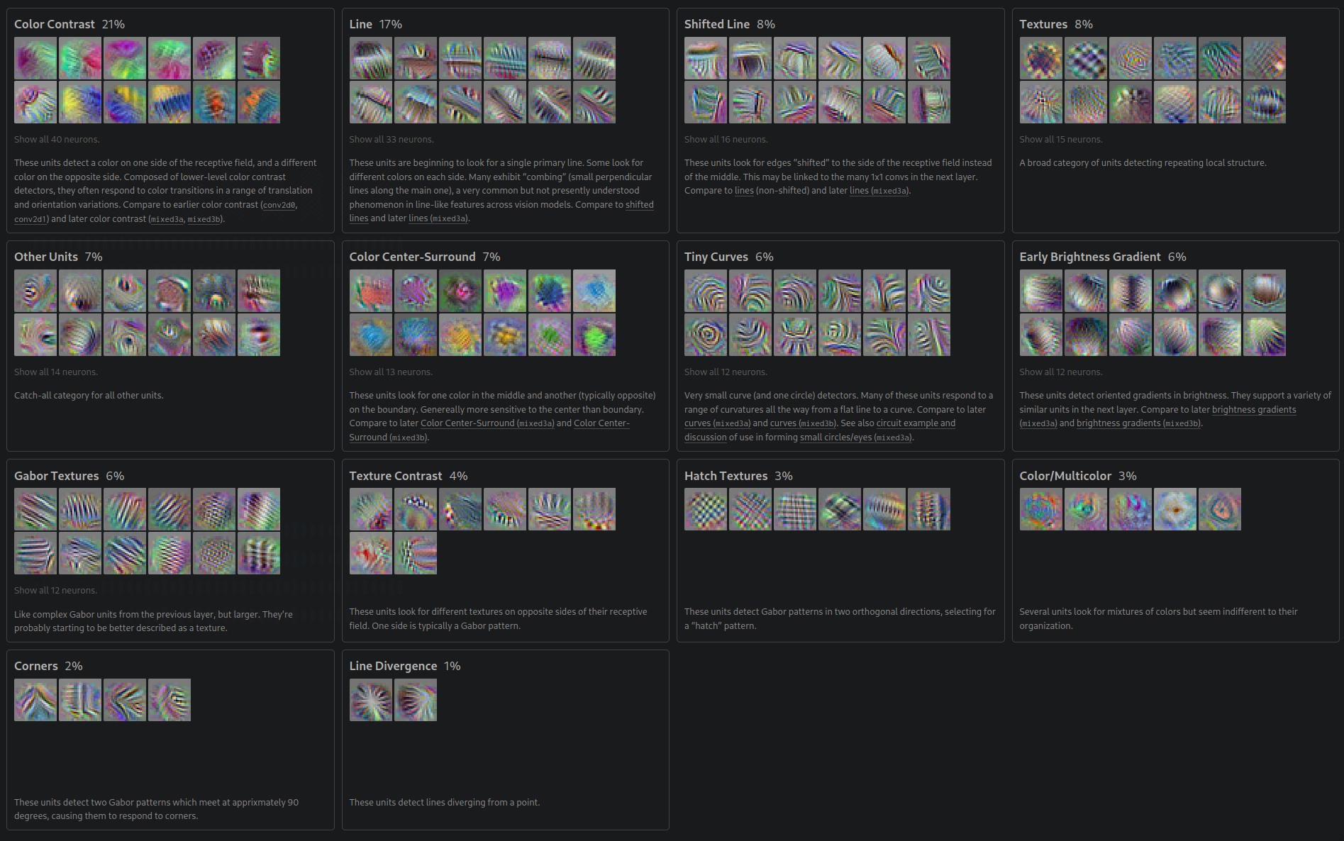
By the third layer, these primitives compose into more complex structures — textures, shifted lines, curves, corners, and hatch patterns:
By layer four, recognizable object parts emerge — textures, repeating patterns, curves, and what look like early eye and fur detectors:
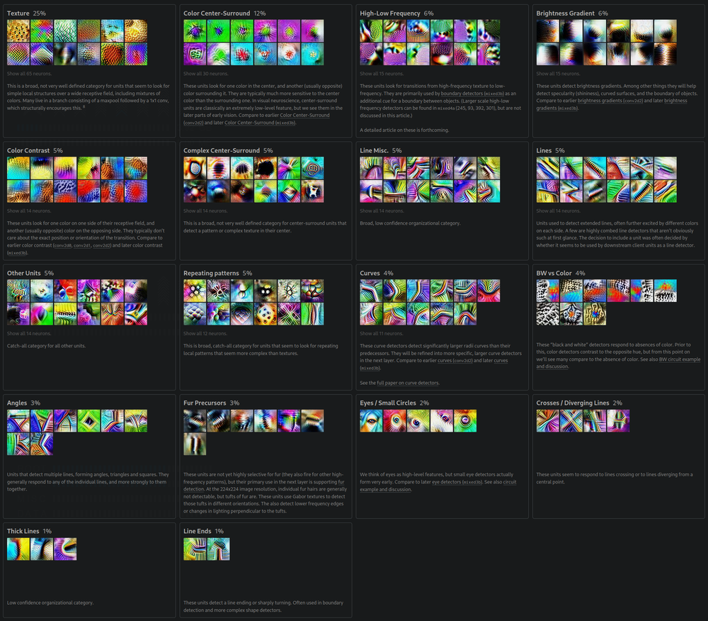
Each layer learns increasingly abstract features. Layer 1 learns edges (Gabor filters). Layer 2 learns textures (combinations of edges). Layer 3 learns object parts. Layer 4 learns objects. The network independently rediscovered the feature hierarchy that vision researchers spent decades designing by hand.
The Winograd Transform
VGGNet established 3x3 as the standard kernel size. ResNet, Inception, and most modern architectures followed. Since the vast majority of convolution operations in practice use 3x3 filters, even modest speedups to 3x3 convolution translate to large real-world gains. Enter Winograd.
Minimal Filtering
The standard approach to computing $m$ output values from a $k$-tap filter requires $m \cdot k$ multiplications. Winograd’s minimal filtering algorithm, based on the Chinese Remainder Theorem, reduces this to $m + k - 1$ multiplications — at the cost of more additions and pre/post-transforms.
For a 3-tap filter ($k = 3$) producing 2 outputs ($m = 2$):
- Direct: $2 \times 3 = 6$ multiplications
- Winograd: $2 + 3 - 1 = 4$ multiplications
This is the $F(2, 3)$ case. Let us work through it.
Worked Example: $F(2, 3)$
Given a filter $\mathbf{g} = [g_0, g_1, g_2]$ and an input tile $\mathbf{d} = [d_0, d_1, d_2, d_3]$, we want to compute:
\[\begin{aligned} y_0 &= g_0 d_0 + g_1 d_1 + g_2 d_2 \\ y_1 &= g_0 d_1 + g_1 d_2 + g_2 d_3 \end{aligned}\]Winograd’s insight is to factor this computation as:
\[\mathbf{y} = A^T \left[ (G\mathbf{g}) \odot (B^T\mathbf{d}) \right]\]where $\odot$ denotes elementwise (Hadamard) multiplication, and the transform matrices for $F(2, 3)$ are:
\[B^T = \begin{bmatrix} 1 & 0 & -1 & 0 \\ 0 & 1 & 1 & 0 \\ 0 & -1 & 1 & 0 \\ 0 & 1 & 0 & -1 \end{bmatrix}, \quad G = \begin{bmatrix} 1 & 0 & 0 \\ \frac{1}{2} & \frac{1}{2} & \frac{1}{2} \\ \frac{1}{2} & -\frac{1}{2} & \frac{1}{2} \\ 0 & 0 & 1 \end{bmatrix}, \quad A^T = \begin{bmatrix} 1 & 1 & 1 & 0 \\ 0 & 1 & -1 & -1 \end{bmatrix}\]The Winograd pipeline: transform filter and input tile, multiply elementwise (the only multiplications), then transform to get the output.
The key observation: the only multiplications in the entire computation are the $m + k - 1 = 4$ elementwise products in the middle step. Everything else — the transforms $G$, $B^T$, and $A^T$ — involves only additions and subtractions. Since the filter transform $G\mathbf{g}$ can be precomputed once per filter, the per-tile cost at inference time is just the input transform, 4 multiplications, and the output transform.
Numerical verification. Let $\mathbf{g} = [1, 2, 3]$ and $\mathbf{d} = [1, 2, 3, 4]$.
Direct computation:
- $y_0 = 1 \cdot 1 + 2 \cdot 2 + 3 \cdot 3 = 14$
- $y_1 = 1 \cdot 2 + 2 \cdot 3 + 3 \cdot 4 = 20$
Winograd:
- $G\mathbf{g} = [1, \, 3, \, 1, \, 3]^T$
- $B^T\mathbf{d} = [-2, \, 5, \, 1, \, -2]^T$
- $(G\mathbf{g}) \odot (B^T\mathbf{d}) = [-2, \, 15, \, 1, \, -6]^T$
- $A^T[-2, \, 15, \, 1, \, -6]^T = [14, \, 20]^T$ $\checkmark$
Extension to 2D
For images, we need 2D convolution. The Winograd transform extends naturally — apply the transforms along both rows and columns:
\[Y = A^T \left[ (G \, g \, G^T) \odot (B^T \, d \, B) \right] A\]where $g$ is now the 2D filter and $d$ is an input tile. The same principle applies: the only multiplications are the elementwise product in the transformed domain.
For $F(2 \times 2, \, 3 \times 3)$ — computing a $2 \times 2$ output tile from a $3 \times 3$ filter over a $4 \times 4$ input tile:
- Direct: $2^2 \times 3^2 = 36$ multiplications
- Winograd: $(2 + 3 - 1)^2 = 16$ multiplications — a 2.25x reduction
For $F(4 \times 4, \, 3 \times 3)$:
- Direct: $4^2 \times 3^2 = 144$ multiplications
- Winograd: $(4 + 3 - 1)^2 = 36$ multiplications — a 4x reduction
The trade-off: larger tiles mean greater speedups, but the transform matrices grow and numerical precision degrades. In practice, $F(4 \times 4, \, 3 \times 3)$ hits the sweet spot — the $6 \times 6$ transforms are manageable and the 4x multiplication reduction is substantial.
Winograd is the opposite of the Bitter Lesson. It is a hand-designed algorithmic optimization, not a learned one. But it operates at a level where mathematical structure genuinely helps: the arithmetic of small convolutions is fixed and well-understood. The transforms are exact, not approximate. Sometimes, careful engineering and careful learning are complementary.
Implementation Details
The gap between textbook convolution and what actually runs on hardware is substantial. Three engineering decisions dominate real-world performance.
Memory Layout: NCHW vs NHWC
A 4D tensor of images has four axes: batch (N), channels (C), height (H), and width (W). The order in which these are laid out in memory affects cache performance dramatically.
| Layout | Memory Order | Used By | Advantage |
|---|---|---|---|
| NCHW | Batch, Channels, Height, Width | PyTorch, cuDNN (default) | Spatial locality within each channel |
| NHWC | Batch, Height, Width, Channels | TensorFlow, Apple MLX | All channels at a pixel are contiguous |
NCHW is natural for convolution: when a kernel slides across one channel, the spatial values it accesses are contiguous in memory. NHWC is better for pointwise operations across channels (like $1 \times 1$ convolutions). Modern frameworks support both, and some internally transpose for optimal performance.
The im2col Trick
The most widely used implementation strategy does not compute convolution directly at all. Instead, it reduces convolution to a single large matrix multiplication.
im2col (image to column) rearranges each receptive field patch into a column of a matrix. If we have a $3 \times 3$ kernel sliding over a $5 \times 5$ image, each of the $3 \times 3 = 9$ overlapping patches becomes a column of length 9. Stack all patches side by side, and reshape the kernels into rows. Now convolution is a single GEMM (General Matrix Multiply) call.
im2col converts convolution to matrix multiplication. Each image patch becomes a column; each filter becomes a row. One GEMM computes all outputs.
The trade-off: im2col duplicates data (overlapping patches share pixels), increasing memory usage. But GEMM is so aggressively optimized — decades of BLAS engineering, hardware-specific microkernel implementations — that this approach consistently wins in practice.
GPU Algorithm Selection
In practice, NVIDIA’s cuDNN library does not commit to a single algorithm. It selects from multiple implementations based on the specific input dimensions:
- Direct convolution — straightforward, good for unusual sizes
- FFT-based — wins for large kernels
- Winograd — wins for 3x3 kernels on Volta+ architectures
- Implicit GEMM — im2col fused into the GEMM kernel to avoid the memory overhead
Setting torch.backends.cudnn.benchmark = True enables autotuning: cuDNN benchmarks each algorithm on the first forward pass and caches the fastest choice for each input shape.
Backpropagation Through Convolution
A beautiful fact connects this post to Autodifferentiation: the gradient of a convolution with respect to the input is itself a convolution — with the kernel flipped (rotated 180 degrees). Similarly, the gradient with respect to the kernel is a convolution of the input with the upstream gradient. This means the same optimized convolution machinery (im2col, Winograd, cuDNN) can be reused for both the forward and backward passes.
What’s Next
We have traced an arc from hand-designed kernels through learned features to the mathematical and engineering optimizations that make convolution fast in practice. The interplay is striking: the Bitter Lesson tells us to learn everything, yet Winograd and im2col — hand-designed, mathematically grounded optimizations — deliver real speedups precisely because the arithmetic of small convolutions is fixed and well-understood. Both careful learning and careful engineering matter.
CNNs bet on spatial locality — nearby pixels matter more than distant ones. But what if every position should attend to every other position equally? That is the opposite bet, and it is the subject of the next post:
- Take Heed of the Hydra covers the transformer architecture, where self-attention replaces convolution entirely — and where the challenge shifts from spatial structure to sequence-length scaling
Vision Transformers (ViT) later showed that these two approaches can be synthesized: patch an image into a sequence of tokens, then apply self-attention. The inductive bias of locality is not baked into the architecture — it is learned from data. The Bitter Lesson strikes again.