We build autodifferentiation (AD) from the ground up. Having a deep understanding of AD is essential for anyone doing serious deep learning research — it’s the mechanism that makes training neural networks possible, and understanding it transforms how you think about computation itself.
What This Post Covers
- Modeling & Objective Functions — Why we need to optimize, and what we’re optimizing
- The Calculus of Optimization — Derivatives, gradients, and why they act as a compass
- Forward Mode AD — Computational graphs traversed leaf-to-root, with a worked example
- Reverse Mode AD (Backpropagation) — Root-to-leaf traversal, adjoint variables, and why reverse mode dominates deep learning
- Loss Functions & Maximum Likelihood — Connecting AD to the functions we actually differentiate
- Gradient Descent, SGD, & Momentum — Putting gradients to work
- Implementation — A minimal autodiff engine in Python
Why Build It From Scratch?
Frameworks like PyTorch and JAX abstract away the differentiation machinery. This is powerful for productivity, but dangerous for understanding. When your gradients explode, vanish, or produce NaN — and they will — you need a mental model of what’s actually happening inside loss.backward(). Building AD from scratch gives you that model.
Predicting the Future
The question that drives all of machine learning is deceptively simple: can we predict what happens next?
To predict, we need to model — to build approximate descriptions of the world around us. Take a snapshot of the world as a collection of objects and their states:
\[\text{World} = \{(\text{Object}, \text{State})\}\]Phenomena — physics, economics, psychology — are functions that transform the world from one state to the next. We’ve developed remarkably accurate formulas for many of these phenomena, but how did we get them?
Divine intervention may have worked for Ramanujan, but the rest of us are forced to learn from data. We perform experiments, record results, and try to extrapolate patterns. Galileo demonstrated this beautifully — Aristotle had claimed that heavier objects fall faster, that twice the weight falls twice as fast. Galileo simply ran the experiment and proved it wrong.
The simplest version of learning from data is linear regression. Given some observations, fit a line:
\[Y_i = \beta_0 + \beta_1 X_i\]where $\beta_0$ is the intercept and $\beta_1$ is the slope. But how do we find the best $\beta_0$ and $\beta_1$? We need a way to measure “best.”
Objective Functions
We’re looking for a good guess of the function determining the behavior of a system, as measured by some accuracy criterion — also called an objective function.
Consider fitting data that looks like a parabola. We might guess the general structure is a second-order polynomial: $y = ax^2 + bx + c$. The choice of this structure is a hyperparameter — a decision we make before training. The variables $a$, $b$, $c$ are parameters — knobs we tune to select a specific member from that family of functions.
To measure how wrong our guess is, we need a loss function. A natural choice is Mean Squared Error:
\[\text{MSE} = \frac{1}{n}\sum_{i=1}^{n}(y_i - \hat{y}_i)^2\]This penalizes large errors more than small ones (thanks to the squaring) and gives us a single number summarizing our model’s performance. Our objective: minimize this quantity.
How can we brute-force a good guess for the parameters? Computers are good at brute-forcing things, so let’s let them do the heavy lifting:
- Start with a random initial guess
- Gauge the performance of the guess
- Perturb the parameters and compare — if the new guess is better, keep it; if not, toss it
- Repeat until satisfied
This works in principle, but it’s wildly inefficient. Randomly poking at parameters in high-dimensional space is like trying to find the lowest point in a mountain range by wandering with a blindfold on. We need a smarter approach — we need to know which direction is downhill.
A Detour Through Calculus
The derivative of a function is the instantaneous rate of change at a point. It measures how rapidly the function is changing — when you nudge $x$ slightly, how much does $f(x)$ change?
\[\frac{df}{dx} = \lim_{h \to 0} \frac{f(x + h) - f(x)}{h}\]A multivariable function takes several inputs, like $f(x, y, z) = ax + by + cz$. A partial derivative with respect to one variable is found by holding all other variables constant and differentiating normally. For example, $\frac{\partial f}{\partial x} = a$.
The gradient collects all the partial derivatives into a single vector:
\[\nabla f = \left[\frac{\partial f}{\partial x}, \frac{\partial f}{\partial y}, \frac{\partial f}{\partial z}\right]\]Here’s the key insight: the gradient points in the direction of steepest ascent. To find a minimum, we walk the opposite way. Minima occur where the derivative transitions from negative to positive — the function stops decreasing and starts increasing.
The gradient is a compass — it always points uphill. To descend, walk the other way.
But there’s a catch. Our objective functions are multivariable functions of potentially millions of parameters. Computing the gradient efficiently is the whole game. This is where automatic differentiation enters.
Neural Networks in One Page
Before we get to AD, let’s establish what we’re differentiating. Shallow neural networks are functions $y = f[\mathbf{x}, \boldsymbol{\phi}]$ with parameters $\boldsymbol{\phi}$ that map multivariate inputs $\mathbf{x}$ to multivariate outputs $\mathbf{y}$ — mapping an $n$-dimensional data space to a $K$-dimensional class space.
A shallow network computes:
\[y = \varphi_0 + \varphi_1 \, a[\theta_{10} + \theta_{11} x] + \varphi_2 \, a[\theta_{20} + \theta_{21} x] + \varphi_3 \, a[\theta_{30} + \theta_{31} x]\]where $a[\cdot]$ is an activation function — a nonlinearity applied to each hidden unit. A common choice is the Rectified Linear Unit (ReLU):
\[\text{ReLU}(z) = \max(0, z) = \begin{cases} 0 & z < 0 \\ z & z \geq 0 \end{cases}\]The ReLU activation function: zero for negative inputs, identity for positive inputs.
Each layer of a neural network is a matrix multiplication followed by an activation. The whole network is a chain of these operations — a deeply nested composition of functions.
A shallow neural network with 3 inputs, 4 hidden units, and 2 outputs. Every connection carries a learnable weight.
The Universal Approximation Theorem tells us that for any continuous function, there exists a shallow network that can approximate it to any desired precision. The catch is that the network might need to be absurdly wide — deep networks achieve the same expressiveness far more efficiently.
The Chain Rule
Neural networks are compositions of functions — layer after layer of linear transformations and nonlinearities. To find the gradient of the loss with respect to every parameter, we need a way to differentiate through this entire chain. Enter the chain rule.
Let $f = f(x, y)$ where $x = x(t)$ and $y = y(t)$. Then:
\[\frac{df}{dt} = \frac{\partial f}{\partial x}\frac{dx}{dt} + \frac{\partial f}{\partial y}\frac{dy}{dt}\]The chain rule decomposes the derivative of a composite function into a product of derivatives of its parts. For a deep network with millions of parameters, we need to apply this rule recursively through every layer.
There are three approaches to computing these derivatives:
Numerical differentiation approximates the derivative with finite differences: $\frac{f(x+h) - f(x)}{h}$. It’s simple but slow (requires two function evaluations per parameter) and numerically unstable (too-small $h$ causes floating-point cancellation, too-large $h$ gives inaccurate approximations).
Symbolic differentiation applies calculus rules to produce exact derivative expressions. It works, but expressions grow exponentially with depth — a phenomenon called expression swell. For a deep network, the symbolic derivative can be vastly larger than the original function.
Automatic differentiation is the sweet spot. It computes exact derivatives (no approximation error) at a cost proportional to the original computation (no expression swell). It works by decomposing every function into elementary operations and applying the chain rule at each step.
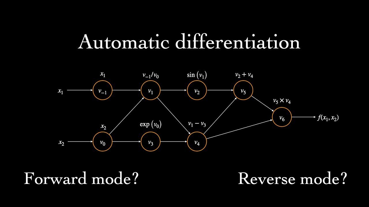
Automatic Differentiation
AD constructs a computational graph for your objective function — a directed acyclic graph where each node is an elementary operation and edges represent data flow. This graph bookkeeps the relationships of the various inner functions with one another.
There are two primary modes of traversal.
Forward Mode
In forward mode, the graph is traversed from leaf nodes to the root. At each node, we compute both the value and the derivative with respect to a chosen input variable, propagating both forward through the graph.
Worked example. Consider $e = (a \cdot b) \cdot (b + 1)$ where $a{=}2$ and $b{=}3$. We want both $\frac{\partial e}{\partial a}$ and $\frac{\partial e}{\partial b}$.
First, decompose into elementary operations:
- $c = a \cdot b$
- $d = b + 1$
- $e = c \cdot d$
Computational graph for e = (a·b)·(b+1). Each edge is annotated with the local partial derivative.
To compute $\frac{\partial e}{\partial a}$, we propagate forward. The derivative of the product operation $c = a \cdot b$ with respect to one operand is the other operand. The derivative of the addition $d = b + 1$ is always 1.
| Node | Value | $\frac{\partial \cdot}{\partial a}$ | Rule |
|---|---|---|---|
| $a$ | 2 | 1 | seed |
| $b$ | 3 | 0 | constant w.r.t. $a$ |
| $c = a \cdot b$ | 6 | $b = 3$ | product rule |
| $d = b + 1$ | 4 | 0 | no path from $a$ |
| $e = c \cdot d$ | 24 | $d \cdot 3 + c \cdot 0 = 12$ | chain rule |
So $\frac{\partial e}{\partial a} = 12$. By the same procedure with $b$ seeded to 1 instead, $\frac{\partial e}{\partial b} = 4 \cdot 2 + 6 \cdot 1 = 14$.
The catch: forward mode computes derivatives with respect to one input per pass. If you have $n$ parameters and 1 output, you need $n$ passes. For deep learning, where $n$ can be in the millions, this is prohibitively expensive.
Reverse Mode
Reverse mode traverses the graph in the opposite direction: from root to leaf nodes. Instead of asking “how does this input affect the output?”, it asks “how does the output depend on each intermediate value?”
We define the adjoint of each node $v_i$ as $\bar{v}_i = \frac{\partial e}{\partial v_i}$ — the sensitivity of the final output to changes in that intermediate value. We start at the root ($\bar{e} = 1$, since $\frac{\partial e}{\partial e} = 1$) and propagate backward.
Worked example. Let $V = xy + z(x + y)$ with inputs $x$, $y$, and $z$.
Decompose into elementary operations:
- $w_1 = xy \to f_1(x, y)$
- $w_2 = x + y \to f_2(x, y)$
- $w_3 = w_2 \cdot z \to f_3(w_2, z)$
- $V = w_1 + w_3 \to f_4(w_1, w_3)$
Computational graph for V = xy + z(x+y). Reverse mode propagates adjoints from the root backward to the leaves.
Applying the chain rule backward:
\[dV = \frac{\partial f_4}{\partial w_1} df_1 + \frac{\partial f_4}{\partial w_3} df_3\]Expanding $df_1$ and $df_3$ in terms of the inputs:
\[dV = \frac{\partial f_4}{\partial w_1}\left(\frac{\partial f_1}{\partial x}dx + \frac{\partial f_1}{\partial y}dy\right) + \frac{\partial f_4}{\partial w_3}\left(\frac{\partial f_3}{\partial w_2}\left(\frac{\partial f_2}{\partial x}dx + \frac{\partial f_2}{\partial y}dy\right) + \frac{\partial f_3}{\partial z}dz\right)\]Since $\frac{\partial f_4}{\partial w_1} = 1$, $\frac{\partial f_4}{\partial w_3} = 1$, $\frac{\partial f_1}{\partial x} = y$, $\frac{\partial f_1}{\partial y} = x$, $\frac{\partial f_3}{\partial w_2} = z$, $\frac{\partial f_2}{\partial x} = 1$, $\frac{\partial f_2}{\partial y} = 1$, and $\frac{\partial f_3}{\partial z} = w_2 = x + y$:
\[\frac{\partial V}{\partial x} = y + z, \quad \frac{\partial V}{\partial y} = x + z, \quad \frac{\partial V}{\partial z} = x + y\]The crucial insight: reverse mode computes derivatives with respect to all inputs in a single pass. Forward mode computes one column of the Jacobian per pass; reverse mode computes one row. For a scalar loss function $L: \mathbb{R}^n \to \mathbb{R}$ — which is exactly what we have in deep learning — reverse mode gets all $n$ partial derivatives in one backward pass. This is why backpropagation is reverse-mode AD, and why it dominates neural network training.
In ML, our computational graph vertices are not scalars and scalar functions — they are matrices, matrix products, and pointwise nonlinear functions. We’re handwaving over the world of matrix differential calculus, but the principle is the same.
What Are We Differentiating? Loss Functions
AD gives us efficient gradients, but gradients of what? In supervised learning, we’re differentiating a loss function that measures the gap between our model’s predictions and observed data.
The principled way to construct loss functions is through maximum likelihood. The model computes distribution parameters $\boldsymbol{\theta}_i = f[\mathbf{x}_i, \boldsymbol{\phi}]$ for each input, and each output $y_i$ should have high probability under its corresponding distribution $\Pr(y_i \mid \boldsymbol{\theta}_i)$. We choose parameters $\boldsymbol{\phi}$ to maximize the combined probability across all $I$ training examples:
\[\hat{\boldsymbol{\phi}} = \underset{\boldsymbol{\phi}}{\text{argmax}} \prod_{i=1}^{I} \Pr(y_i | f[\mathbf{x}_i, \boldsymbol{\phi}])\]This product is the likelihood of the parameters. Two assumptions lurk here: the data are identically distributed (same form for each data point) and the conditional distributions are independent (i.i.d.).
Taking the product of many small probabilities is numerically unstable — underflow is guaranteed. A nice property of logarithms saves us: $\log(xy) = \log x + \log y$. Since $\log$ is monotonically increasing, maximizing the log-likelihood is equivalent to maximizing the likelihood:
\[\hat{\boldsymbol{\phi}} = \underset{\boldsymbol{\phi}}{\text{argmax}} \sum_{i=1}^{I} \log \Pr(y_i | f[\mathbf{x}_i, \boldsymbol{\phi}])\]By convention, we frame optimization as minimization (descending a loss surface). Negating the log-likelihood gives us the loss:
\[\hat{\boldsymbol{\phi}} = \underset{\boldsymbol{\phi}}{\text{argmin}} \left[ -\sum_{i=1}^{I} \log \Pr(y_i | f[\mathbf{x}_i, \boldsymbol{\phi}]) \right] = \underset{\boldsymbol{\phi}}{\text{argmin}} \, L[\boldsymbol{\phi}]\]The recipe for constructing loss functions:
- Choose a suitable probability distribution $\Pr(\mathbf{y} \mid \boldsymbol{\theta})$ over the domain of predictions
- Set the model to predict one or more distribution parameters: $\boldsymbol{\theta} = f[\mathbf{x}, \boldsymbol{\phi}]$
- Find $\hat{\boldsymbol{\phi}}$ that minimizes the negative log-likelihood over training pairs $\{(\mathbf{x}_i, \mathbf{y}_i)\}$
- To predict: return the full distribution $\Pr(\mathbf{y} \mid f[\mathbf{x}, \hat{\boldsymbol{\phi}}])$ or its maximum
For Gaussian outputs with fixed variance, this recipe recovers MSE. For Bernoulli outputs (binary classification), it gives binary cross-entropy. The choice of distribution determines the loss.
Gradient Descent
We now have all the pieces: a model (neural network), a loss function (negative log-likelihood), and a way to compute gradients (reverse-mode AD). Gradient descent puts them together.
Step 1. Compute the gradient of the loss with respect to all parameters:
\[\frac{\partial L}{\partial \boldsymbol{\phi}} = \begin{bmatrix} \frac{\partial L}{\partial \phi_0} \\ \frac{\partial L}{\partial \phi_1} \\ \vdots \\ \frac{\partial L}{\partial \phi_N} \end{bmatrix}\]Step 2. Update the parameters by stepping opposite to the gradient:
\[\boldsymbol{\phi} \leftarrow \boldsymbol{\phi} - \alpha \cdot \frac{\partial L}{\partial \boldsymbol{\phi}}\]where the positive scalar $\alpha$ is the learning rate — it determines the step size.
For linear regression, the loss surface is convex: a bowl with a single global minimum. No chord between two points on the surface intersects the function. Convexity guarantees that gradient descent will find the global minimum — the training procedure can’t fail.
Unfortunately, loss functions for most nonlinear models — including neural networks — are non-convex. The landscape is riddled with local minima (valleys that aren’t the deepest), saddle points (flat in some directions, curved in others), and plateaus. The final destination of gradient descent is entirely determined by the starting point.
Stochastic Gradient Descent (SGD) addresses this by adding noise. Instead of computing the gradient over the entire dataset, SGD uses random mini-batches. The solution still moves downhill on average, but the randomness allows it to occasionally move uphill — jumping from one valley of the loss function to another, potentially finding a deeper minimum.
Momentum is a common enhancement: instead of using only the current gradient, we maintain a running average that blends the current gradient with the previous direction of travel:
\[\mathbf{m}_{t+1} \leftarrow \beta \cdot \mathbf{m}_t + (1 - \beta) \sum_{i \in \mathcal{B}_t} \frac{\partial \ell_i[\boldsymbol{\phi}_t]}{\partial \boldsymbol{\phi}}\] \[\boldsymbol{\phi}_{t+1} \leftarrow \boldsymbol{\phi}_t - \alpha \cdot \mathbf{m}_{t+1}\]This smooths out the noisy gradient estimates and helps the optimizer barrel through narrow ravines rather than oscillating between their walls.
Gradient descent on a convex loss surface. Each step follows the negative gradient, with decreasing step sizes as we approach the minimum.
Implementation: A Minimal Autodiff Engine
Let’s build a tiny reverse-mode AD engine in Python. The core idea: wrap every value in a Value object that remembers how it was created (its parents and the operation) so we can retrace the computation during the backward pass.
class Value:
    def __init__(self, data, children=(), op=''):
        self.data = data
        self.grad = 0.0
        self._backward = lambda: None
        self._prev = set(children)
        self._op = op

    def __add__(self, other):
        other = other if isinstance(other, Value) else Value(other)
        out = Value(self.data + other.data, (self, other), '+')
        def _backward():
            self.grad += out.grad       # d(a+b)/da = 1
            other.grad += out.grad      # d(a+b)/db = 1
        out._backward = _backward
        return out

    def __mul__(self, other):
        other = other if isinstance(other, Value) else Value(other)
        out = Value(self.data * other.data, (self, other), '*')
        def _backward():
            self.grad += other.data * out.grad  # d(a*b)/da = b
            other.grad += self.data * out.grad  # d(a*b)/db = a
        out._backward = _backward
        return out

    def relu(self):
        out = Value(max(0, self.data), (self,), 'ReLU')
        def _backward():
            self.grad += (self.data > 0) * out.grad
        out._backward = _backward
        return out

    def backward(self):
        topo = []
        visited = set()
        def build_topo(v):
            if v not in visited:
                visited.add(v)
                for child in v._prev:
                    build_topo(child)
                topo.append(v)
        build_topo(self)
        self.grad = 1.0
        for v in reversed(topo):
            v._backward()

    def __neg__(self):      return self * -1
    def __sub__(self, o):   return self + (-o)
    def __radd__(self, o):  return self + o
    def __rmul__(self, o):  return self * o
    def __repr__(self):     return f"Value(data={self.data}, grad={self.grad})"
The backward() method performs the reverse pass: it topologically sorts the graph (ensuring each node is processed after all its consumers), seeds the root gradient to 1.0, then calls each node’s _backward closure in reverse order.
Let’s verify with our earlier examples:
# Forward example: e = (a*b)*(b+1), a=2, b=3
a = Value(2.0)
b = Value(3.0)
e = (a * b) * (b + 1)
e.backward()
print(f"e = {e.data}, de/da = {a.grad}, de/db = {b.grad}")
# e = 24.0, de/da = 12.0, de/db = 14.0  ✓

# A tiny neural network: y = relu(w1*x + b1) * w2 + b2
x = Value(2.0)
w1, b1 = Value(-3.0), Value(1.0)
w2, b2 = Value(2.0), Value(0.5)
y = ((w1 * x + b1).relu() * w2) + b2
y.backward()
print(f"y = {y.data}, dy/dw1 = {w1.grad}, dy/dw2 = {w2.grad}")
# y = 0.5, dy/dw1 = 0.0, dy/dw2 = 0.0  (ReLU killed the gradient — input was negative!)
This handles scalars only. Extending to tensors — with broadcasting, batched operations, and matrix multiplications — is where frameworks like PyTorch and JAX earn their complexity. But the principle is identical: record, traverse backward, accumulate gradients.
What’s Next
We’ve gone from “predict the future” to a working autodiff engine — the same core algorithm powering every loss.backward() call in PyTorch. If you want to go deeper:
- Convoluted Computation explores convolutions, which have their own efficient gradient computations
- Multihead Attention covers the transformer architecture, where AD handles attention weight gradients across sequence positions
- A future post will extend this scalar engine to tensors, implementing broadcasting and matrix operations from scratch