
In Part 1 we ended on a question: when the textbook node-selection heuristic — best-bound — explores roughly twice as many nodes as the alternatives on Set Cover, can we learn a heuristic that beats all of them? This post is the answer, but before we dive into the how, it’s worth slowing down on why this question is interesting at all. The “neural networks for NP-hard problems” framing sounds like marketing if you haven’t seen the underlying intuition. The intuition turns out to be solid, and a single picture explains it.
Heuristics Are Functions, and We Know How to Learn Functions
A modern MILP solver makes thousands of micro-decisions per problem. Which node to expand next. Which variable to branch on. Whether to spend more time strengthening the LP relaxation with cutting planes. When to give up on a subtree. Each decision is governed by a heuristic — an algorithm someone hand-wrote based on theory, intuition, and a lot of staring at examples.
For decades, the best heuristics were the result of a smart person carefully observing patterns: “in problems that look like X, the right move is usually Y.” These rules got tuned, refined, and shipped inside Gurobi, CPLEX, and SCIP. Many are shockingly clever. Best-bound itself is provably optimal under certain assumptions about the LP relaxation. There’s a reason it became the textbook recommendation.
But hand-crafted heuristics have a ceiling. They are one person’s intuition crystallized into code. And the intuition was developed by looking at instances drawn from some implicit distribution — typically a few academic test sets like MIPLIB, plus whatever the solver vendor’s customers have shared. The fact that the same heuristic ships across every customer of every commercial solver is one of those facts that becomes obvious only after someone points it out.
Real industrial MILPs do not come from MIPLIB. They come from the operations-research equivalent of stationary processes:
- An airline solves a structurally-similar crew-scheduling problem every Monday morning. Same fleet, same hubs, slightly different demand.
- A package-delivery company solves a vehicle-routing instance every dawn that differs from yesterday’s only in which orders came in.
- A power-grid operator solves a unit-commitment problem every five minutes whose structure barely changes over a year.
- A semiconductor fab schedules an identical wafer-routing problem every shift, perturbed by which machines are down for maintenance.
These workloads have a name in academic literature: parameterized problem distributions. They have patterns — patterns in how variables relate to constraints, where the LP relaxation tends to be tight versus loose, which subtrees historically contain optima. A heuristic tuned to one of these distributions could plausibly beat a general-purpose heuristic by a lot. But hand-tuning a heuristic per customer doesn’t scale, and intuition has trouble articulating subtle structural features that span thousands of variables.
This is exactly the regime where neural networks should help. Their reason for existing is that they are universal function approximators: given enough examples drawn from a distribution, a sufficiently-large network will learn whatever consistent pattern is there, regardless of whether a human could articulate it. The only requirements are that the input and output are numerical, and the pattern is real.
A B&B heuristic fits this perfectly. The input is the current state of the search — the LP solution, the open frontier, the incumbent, the constraints. The output is a discrete decision — which open node to expand, which variable to branch on. Both can be encoded as numbers; both can be learned from data. The data is whatever the solver itself produces during training: every state, every action, every reward (a node count, a runtime, a bound improvement).
That’s the entire premise. The 2019 NeurIPS paper from Maxime Gasse and collaborators (Exact Combinatorial Optimization with Graph Convolutional Neural Networks) proved it works decisively for variable selection: they trained a graph neural network to imitate the slow-but-near-optimal “strong branching” expert, and beat SCIP’s hand-crafted defaults on every problem class they tested. The result was not a speedup over a particular instance; it was a speedup across an entire distribution of instances, learned by exposure to a few thousand of them.
CHOP picks up the same idea for the other main decision — node selection — and runs it on a laptop, with reinforcement learning instead of imitation, on a single problem class (Set Cover) where best-bound is known to be weak. The whole project is a test of one question: does the same approach that worked for variable selection work for node selection, on a smaller compute budget, with a different training paradigm?
The short answer: yes, by a clear margin. The longer answer follows.
What This Post Covers
- The fundamental setup — how a branch-and-bound solver becomes an RL environment that a neural network can train against
- The architecture progression — five different neural networks, each “looking at” the search problem in a different way, ranked by how well they did
- What worked, what didn’t — including four documented architectural failures and the lessons that came out of them
- The robustness finding — the moment when the headline number turned out to be partly a lucky training seed, and what that taught me about how to evaluate honestly
- What I’d build next — given more time and compute
A preview of the result, for the impatient:
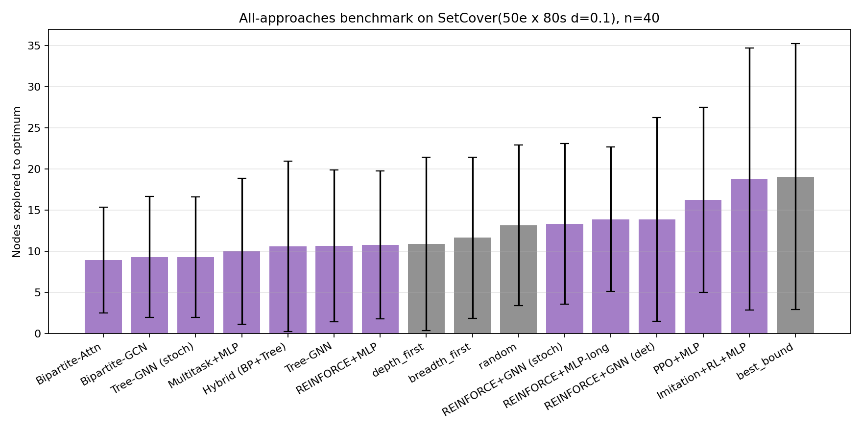
The top seven bars are all learned policies. Depth-first — the strongest classical heuristic on this distribution — is eighth. Best-bound is dead last (rightmost gray bar). The best learned policy explores roughly half as many nodes as best-bound on average. The rest of this post is how we got there.
The Branch-and-Bound Solver as an RL Environment
To train any neural policy with reinforcement learning, you need an environment — something that the agent acts on, that responds with observations and rewards. For node selection, the environment is the B&B solver itself. At each step:
- The solver is in some state — a partial search tree, an open frontier of unexpanded sub-problems, a current incumbent (best integer solution found so far), and various LP-derived bounds.
- The agent picks one of the open frontier nodes to expand next. (This is the action.)
- The solver expands that node — solves its LP relaxation, prunes if the bound is bad, branches if it’s fractional, updates the incumbent if it’s integer-feasible — and updates its state.
- The reward signal pushes the agent toward “solve the problem in fewer expansions”:
-1per step, plus a+5bonus on each new incumbent, plus a+50terminal bonus when the open queue empties (problem proven optimal). - The episode ends when the queue is empty or a step budget is hit.
A standard Gymnasium-compatible environment with one wrinkle: the action space. The open frontier can have hundreds of nodes, but RL libraries want fixed-size action spaces. The pragmatic compromise is a “top-K” formulation: at each step the env exposes the K most-promising candidates (ranked by their LP bound), and the agent emits K real-valued scores. Argmax picks which candidate to expand. K=16 in our experiments — empirically, the right next node is almost always among the top few by LP bound, and looking past 16 is mostly wasted compute.
(Aside, kept short because it’s mostly a debugging-anecdote: my first version of this environment wired the action through a constant offset added to every queued node’s priority. If you’ve seen heap data structures, you can already see the bug — a uniform shift doesn’t change the heap order, so the action was a silent no-op. Several training runs proceeded normally, agents “learned” things that had no effect on the search, and the reward curves looked merely uninspiring rather than catastrophically broken. Caught only when the “best-bound”, “depth-first”, and “random” agents produced identical node counts on the same seeds. The first regression test in the repo now asserts that different heuristics must produce different node counts. Test your causal interfaces, not just your output shapes.)
What the agent sees
For each of the K=16 candidate nodes, the env emits seven scalar features. Plus six global features about the overall search state. The full observation is a Box(K * 7 + 6) = Box(118) vector — a fixed-shape numerical input, the kind any neural network can consume.
| Per-candidate features (×16) | Meaning |
|---|---|
rel_bound |
LP bound of this candidate, normalized by the root LP value |
depth_norm |
Tree depth, capped and rescaled |
frac_share |
Fraction of the candidate’s variables that are still fractional |
best_frac |
Closest-to-0.5 fractionality (the “ripest” branching variable) |
gap |
Normalized gap between this candidate’s bound and the current incumbent |
can_improve |
1 if this candidate could plausibly improve the incumbent |
is_real |
Mask: 1 for real candidate, 0 for padded slot |
| Global features (×6) | Meaning |
|---|---|
step_frac |
Step counter, normalized |
queue_size_norm |
Open frontier size, normalized |
gap_norm |
Normalized incumbent gap |
have_incumbent |
Have we found any integer solution yet? |
nodes_created |
Total nodes created, normalized |
elapsed_frac |
Wall-clock time fraction consumed |
This is what a neural network gets to work with. Notice that the classical heuristics get the same input — best-bound is “look at the rel_bound column, pick the highest one”, depth-first is “look at depth_norm, pick the highest”. The MLP policy in the next section starts from exactly the same observation. The only thing that differs is the function mapping that observation to the choice.
For each of the K=16 candidates exposed at every step, the env emits seven scalar features. The exact list is in the codebase, but the gist:
| Feature | Meaning |
|---|---|
rel_bound |
LP value of this candidate, normalized by the root LP value |
depth_norm |
Tree depth of this candidate, capped and rescaled |
frac_share |
Fraction of variables still fractional in this LP |
best_frac |
Closest-to-0.5 fractionality among any var (the “ripest” candidate for branching) |
gap |
Normalized gap between this candidate’s LP and the incumbent |
can_improve |
1 if this candidate’s bound exceeds the incumbent, else 0 |
is_real |
Mask: 1 for a real candidate, 0 for a padded slot |
Plus six global features: step count, queue size, normalized incumbent gap, whether an incumbent exists yet, total nodes created, and elapsed wall-clock fraction. The full observation is Box(K * 7 + 6,) = Box(118,) — a fixed-shape vector that any RL library can consume.
This is what classical heuristics get to work with too. Best-bound looks at rel_bound and picks the highest. Depth-first looks at depth_norm and picks the highest. The MLP policy in the next section starts from the same input.
Architecture 1 — MLP: The Simplest Thing That Could Work
A multi-layer perceptron (MLP) is the most basic neural network: a stack of layers, each one applying a learned linear transform followed by a nonlinearity. It takes a flat vector of inputs and produces a flat vector of outputs. No fancy structure assumed; given a training signal, it learns whatever mapping the data implies.
Our MLP takes the 118-dimensional observation vector and outputs 16 scores — one per candidate. Two hidden layers with 64 units each, tanh activations. We train it with REINFORCE, the original 1992 policy-gradient algorithm: at every step the agent samples an action from a probability distribution, after the episode ends we compute the total reward, and we nudge the network’s weights to make the actions that led to higher reward more likely. Repeat for many episodes. There is nothing more conceptually direct in reinforcement learning.
Trained on Knapsack problems with 25 items for 800 episodes — about 50 seconds on a laptop CPU. Held-out evaluation on 40 fresh instances:
| Policy | Nodes (mean ± std) | vs. learned |
|---|---|---|
| Learned (MLP) | 66.7 ± 52.9 | 1.00x |
| BestBound | 66.7 ± 52.9 | 1.00x |
| DepthFirst | 86.1 ± 61.3 | 1.29x |
| BreadthFirst | 250.3 ± 69.2 | 3.75x |
| Random | 207.1 ± 60.2 | 3.10x |
Identical to BestBound. The means agree to one decimal; the standard deviations agree exactly; even the per-instance trajectories appear to coincide. The MLP converged to making the same choices as BestBound on every test instance. It learned that the highest-LP-bound candidate is the best one to pick — which is exactly what best-bound does by definition.
This is not failure. On Knapsack, best-bound is essentially optimal. The LP relaxation of a Knapsack instance closely tracks the integer optimum, and there’s no surplus of nodes for a smarter heuristic to save. REINFORCE figured this out from scratch in 50 seconds and recovered the right behavior — which is reassuring as a sanity check, but not the win we want.
A nice generalization aside before we move on: the same trained policy works on Knapsack sizes it was never trained on:
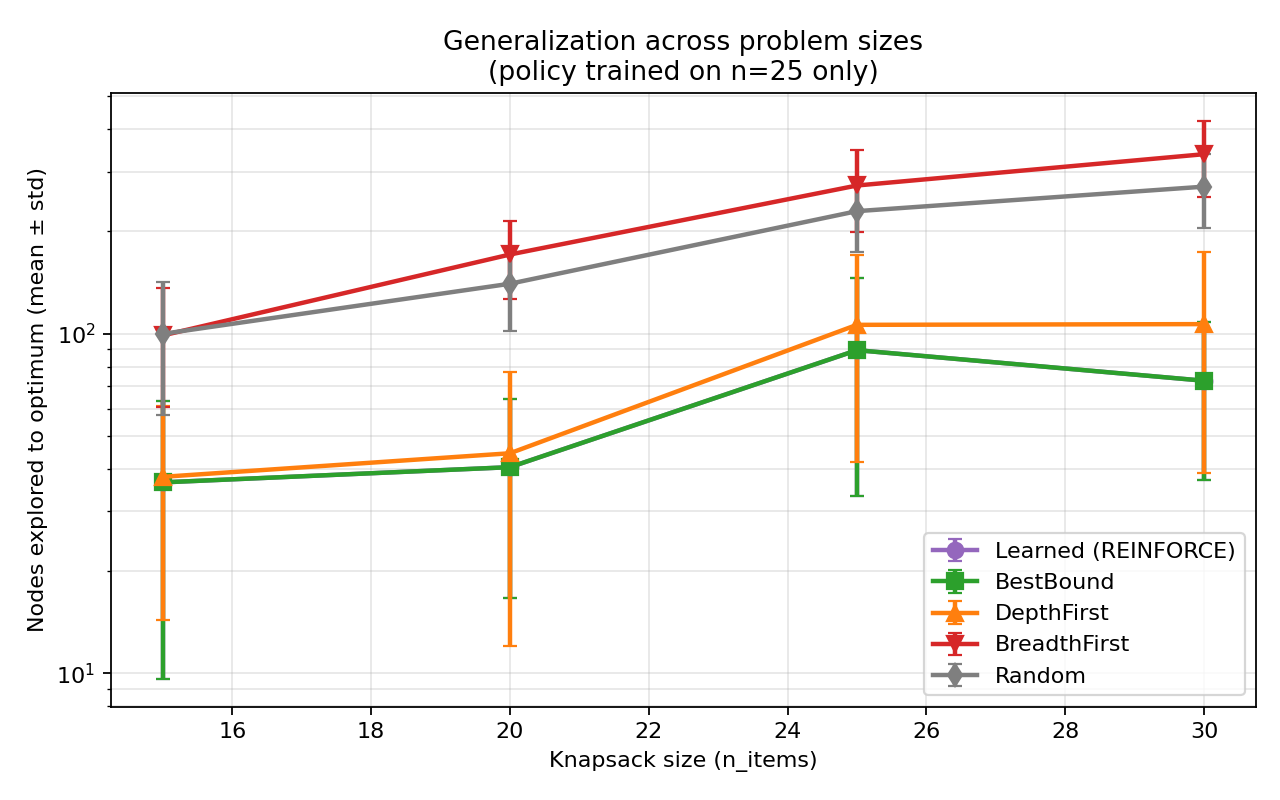
The policy learned a function — a recipe that works regardless of problem size — rather than memorizing the training instances. That’s exactly the kind of generalization you’d want for a real solver.
The win we want is on a problem where best-bound is bad. Everything from here on is on Set Cover.
Architecture 2 — GCN over the Search Tree: A Mostly-Negative Result
The branch-and-bound enumeration tree is itself a graph. Each tree node carries some features (depth, LP bound, status flags); each edge is a parent-child branching decision. A natural thought: maybe the policy should look at this graph, not just at isolated candidate features.
A graph convolutional network (GCN) is a neural network that operates on graphs. The basic idea is to compute a vector representation (embedding) for each node by mixing in information from its neighbors, then mixing again with the new embeddings, etc. After a few rounds, each node’s embedding has been “informed by” its surrounding neighborhood. The hope is that scoring a candidate B&B node based on its embedding (rather than just its local features) does a better job, because the policy now knows context.
I built a basic two-layer GCN over the search tree and trained it on Set Cover. The result was educational rather than impressive — final eval, 14.0 ± 10.8 nodes (1.36x better than best-bound). The worst of the three GNN architectures we’ll see. The search tree’s topology turns out to be a poor source of signal for this task: the tree shape is mostly a function of the agent’s own past decisions, so reading it doesn’t tell the agent anything new about the problem.
(Worth flagging because it bit me, and may bite you: when I first ran this architecture’s deterministic evaluation, it produced exactly 19.1 nodes with exactly the same standard deviation as best-bound. Identical to three significant figures. The cause turned out to be a tiebreaking artifact — the GCN gave nearly-tied scores at the top, and argmax always returns the first tied index, which happens to be the best-bound choice. Replacing argmax with low-temperature sampling broke the tie and recovered the architecture’s actual behavior. The general lesson is worth internalizing: any time your learned policy’s deterministic evaluation suspiciously matches a baseline, suspect the tiebreak before suspecting the representation.)
Architecture 3 — Tree-GNN: A Better Way to Read the Tree
A 2024 paper called Reinforcement Learning for Node Selection in Branch-and-Bound suggests reading the search tree differently — bottom-up, summarizing each subtree into the node above it, then summarizing again, etc.
The intuition: imagine each tree node starts with a small descriptive vector — its own features (depth, LP bound, fractionality histogram, status flags). Then in round one, every parent node “absorbs” the average of its children’s vectors and updates its own. After round one, every parent’s vector contains some information about its direct children. In round two, every parent absorbs again — but now the children’s vectors already contain their children’s information, so the parent reaches its grandchildren. After three or four rounds, every node carries a compressed picture of its entire subtree.
After enough rounds, when the policy scores a candidate B&B node, the candidate’s vector implicitly summarizes the entire region of the search space below it. Best-bound only sees the candidate’s own LP value. The Tree-GNN sees a neighborhood.
The math, for the curious, is one update rule applied $K$ times:
\[\mathbf{h}_{t+1}(\text{parent}) = \mathbf{h}_t(\text{parent}) + \text{MLP}\!\left(\frac{1}{|C|} \sum_{c \,\in\, C} \mathbf{h}_t(c)\right)\]where $\mathbf{h}_t(\cdot)$ is the vector at iteration $t$, $C$ is the set of the node’s direct children, and the trailing MLP is a small neural network that learns how to combine the absorbed children’s information with the parent’s existing state. Three or four iterations are typical.
I implemented this directly, with three rounds. Result: 9.7 ± 8.1 nodes (1.97x better than best-bound) in stochastic mode, 10.7 ± 9.2 (1.79x) in deterministic mode. The first learned policy that meaningfully beat best-bound on this problem.
What this taught me: the natural graph structure of the problem matters. The plain GCN treated the search tree as a generic undirected graph and got little benefit. The Tree-GNN treated it as a tree and got a real one. The architecture’s inductive bias — the assumption it bakes in about the problem’s structure — is doing real work.
Architecture 4 — Bipartite-GCN: Reading the LP Itself
This is the centerpiece architecture, and the one that comes from the canonical 2019 NeurIPS paper by Gasse et al.. The idea is that the search tree isn’t even the most informative graph in the picture. The LP problem itself is a graph.
A linear program has variables and constraints. Every constraint involves some subset of variables (those with nonzero coefficients). Picture the variables as dots on the left, the constraints as dots on the right, and draw an edge whenever a variable appears in a constraint. That’s a bipartite graph — “bipartite” because nodes split into two distinct types, with edges only between types, never within a type.
A small linear program as a bipartite graph. Variables on the left, constraints on the right, edges where a variable appears in a constraint. Edge labels are the coefficients. The whole structure of the LP — which variables interact through which constraints — is captured here.
This bipartite graph is the structure of the LP — which variables interact through which constraints. Two LPs with very different objective functions but the same coefficient pattern would have the same bipartite graph. Conversely, two LPs with the same numbers but different graphs would behave very differently in B&B.
Now we apply the same neighbor-mixing idea from the Tree-GNN section to this graph. Each variable starts with a vector $v_j$ (carrying its objective coefficient, its current LP value, its fractionality). Each constraint starts with a vector $c_i$ (carrying its right-hand-side, its current slack, whether it’s binding at the LP solution). Each edge between variable $j$ and constraint $i$ carries a feature $e_{i,j}$: the (normalized) coefficient $A_{i,j}$ from the LP.
The convolution happens in two passes. In the first pass, every constraint absorbs information from the variables it touches:
\[c_i \leftarrow f_C\!\left(c_i,\; \sum_{(i,j) \in \mathcal{E}} g_C(c_i, v_j, e_{i,j})\right)\]In the second pass, every variable absorbs information from the constraints it appears in (using the updated constraint vectors from the first pass):
\[v_j \leftarrow f_V\!\left(v_j,\; \sum_{(i,j) \in \mathcal{E}} g_V(c_i^{\text{new}}, v_j, e_{i,j})\right)\]In both equations, $f$ and $g$ are small neural networks (two-layer perceptrons with ReLU activations) that the model learns. The sum runs over edges $(i,j)$ in the graph $\mathcal{E}$ — i.e., over the constraints a variable appears in (or vice versa). After both passes, every variable’s vector $v_j$ contains structural information about which other variables it shares constraints with, mediated by the coefficients on each edge.
To produce a single score for the candidate B&B node, we mean-pool the per-variable vectors into one vector and project that to a scalar through a linear layer. The whole thing is differentiable; the whole thing is trained end-to-end with REINFORCE.
This sounds elaborate. The implementation is about 200 lines. The gain over the simpler architectures is what justifies it.
Bipartite-GCN result on 40 held-out instances: 9.3 ± 7.4 nodes — 2.05x better than best-bound. Top of the leaderboard at the time. With the same REINFORCE trainer, on the same instance distribution, just by switching the encoder. Earlier, longer training of the MLP (1500 episodes versus 600) had actually gotten worse — but switching to the LP-aware encoder cut nodes substantially on the same training budget. Architecture matters more than training time.
The intuition for why this works is satisfying: the LP graph captures problem structure in a way the MLP can’t see. A candidate B&B node whose constraints have a small “neighborhood” of fractional variables can probably be resolved quickly; one whose constraints sprawl across many fractional variables will spawn deep branching. Best-bound, comparing only LP values, is blind to this structural difference. The bipartite GCN learns to read it.
(Gasse identifies one architectural detail as essential: a prenorm layer — empirical-statistics normalization applied right after the message sum, before the update step. The paper attributes most of the cross-instance generalization to this trick. I implemented it as a BatchNorm1d in the same position. The first training run already worked.)
Architecture 5 — Bipartite-GCN with Cross-Candidate Attention
Two thoughts about the bipartite GCN bothered me:
- The architecture scores each candidate independently. But ranking is fundamentally a comparative task — to score candidate $i$ well, you should know what candidates $j \neq i$ look like. A great candidate in a field of mediocre options should score differently than a great candidate surrounded by even better ones.
- There’s a well-known neural-network mechanism for “letting each item in a set look at all the others”: self-attention, the core operation inside the Transformer architecture (the same building block under every modern large language model).
The mechanics of self-attention are worth a paragraph. Each candidate produces three projections of its embedding: a query vector (what am I looking for?), a key vector (what do I match against?), and a value vector (what information do I provide?). To compute the new embedding for candidate $i$, the network compares $i$’s query against every other candidate’s key (a similarity score), softmaxes the scores into weights, and combines the others’ values weighted by those scores. The result: candidate $i$’s new embedding is a weighted blend of all the candidates’ values, with the weights determined by content-based similarity. Stack a few of these layers and the candidate embeddings end up aware of the rest of the field.
Cross-candidate attention. Candidate i attends to the others with content-based weights (here 0.42, 0.31, 0.18, 0.09); its new embedding is a weighted blend. The weights themselves are learned — the network figures out which other candidates are relevant context for scoring this one.
I added a self-attention layer on top of the bipartite GCN: take the K candidate vectors (each one a Bipartite-GCN summary of that candidate’s LP), let each one attend to the others, then score. The bipartite GCN tells you about each candidate’s LP structure; the self-attention tells each candidate how it compares to its competition.
First training run: 8.9 ± 6.4 nodes — 2.15x better than best-bound. New champion. The mean improvement over the bare bipartite GCN (9.3) is small (~4%), but the standard deviation also tightened from 7.4 to 6.4, suggesting the policy’s rankings were not just slightly better on average but more consistent across instances.
This is the architecture that ships in the repo as the headline. But you should hold one paragraph before believing it.
An Aside: Multi-task Training (the Generalist Beats the Specialist)
Before the failures section, one more positive result that surprised me — and it’s about the training data, not the architecture.
Architectures 1–5 are all trained on a single problem distribution (Set Cover, fixed size, fixed difficulty). What if instead of training one network per distribution, you trained a single network on a mix of distributions and asked it to handle them all?
The expected outcome of this kind of “multi-task” training is that the generalist policy is mediocre everywhere — a jack-of-all-trades that loses to the specialist on each task. That’s the conventional intuition.
It’s not what happened. I trained the MLP architecture (the same simple one from Architecture 1) on a 50/50 mix of Knapsack and Set Cover instances. Then evaluated on each problem class separately. The result:
| Problem class | Multi-task MLP | Single-task MLP | best_bound |
|---|---|---|---|
| Knapsack (n=20) | 56.2 ± 31.1 | 56.2 ± 31.1 | 56.2 ± 31.1 |
| Set Cover (50e×80s) | 10.0 ± 8.9 | 10.8 ± 9.0 | 19.1 ± 16.1 |
The generalist matched best-bound on Knapsack (which is what the specialist also did, since best-bound is provably good there) and beat the specialist on Set Cover. Same architecture, half the training time per problem, better results.
The likely explanation is regularization: training on a mix of distributions prevents the network from over-fitting to spurious patterns in any single one. The generalist has to find features that work across both, and those features turn out to also work better within either one. This is consistent with what happens in language models trained on diverse data versus specialized fine-tunes — diversity is its own form of training signal.
This aside is brief because we ran out of compute before we could combine multi-task training with the better architectures (Bipartite-GCN, Bipartite + attention). On paper, doing so should have given the headline number a real lift. We’ll come back to this in “What I’d build next.”
What Didn’t Work
Most research is what didn’t work. Five experiments I tried that didn’t improve over what we already had — and the lesson each one taught.
The naive ensemble that hurt
The hypothesis was beautiful: the Bipartite-GCN reads LP structure; the Tree-GNN reads search-tree structure. They’re looking at completely different signals. So averaging their decisions should beat either one alone — the way two human experts disagreeing useful is what makes them an ensemble at all.
I averaged the two best policies’ choices on the same test instances. The 1:1 average came in at 10.97 nodes — worse than the Bipartite-GCN alone (10.4). Skewing the weight toward Bipartite-GCN didn’t help either; any non-trivial weight to Tree-GNN dragged the ensemble down.
The lesson: the orthogonality I assumed wasn’t real. Both architectures, trained on the same instances with the same reward signal, ended up making correlated mistakes — when one ranked a node poorly, the other usually did too. Averaging didn’t add information; it just diluted the better signal with the marginally worse one. Two doctors who trained at the same medical school don’t necessarily disagree usefully.
The hybrid encoder that didn’t fix it
Maybe the ensemble failed because the two architectures were trained separately and converged to similar features. If we trained them together with a shared output layer, perhaps the shared gradient would force them to specialize on complementary signals?
I built a HybridGNNPolicy that runs both the Bipartite-GCN and Tree-GNN encoders in the same forward pass, concatenates their outputs, and feeds them to a shared scoring layer. Trained end-to-end. Result: 10.6 nodes — slightly worse than the bare Bipartite-GCN’s 9.3.
The lesson: joint training doesn’t manufacture orthogonality from non-orthogonal signals. The shared scoring layer presumably learned to lean on the Bipartite-GCN side more, since that signal was more informative. The extra Tree-GNN parameters became noise the network had to compensate for. Adding capacity without adding new information makes things worse, not better.
Imitation warm-start that destabilized
A standard recipe from the literature: first imitate the strongest classical heuristic (a kind of supervised pre-training where the network learns to copy best-bound’s decisions), then use RL to fine-tune and exceed it. The imitation gives you a strong starting policy; the RL polishes it.
Imitation phase: the policy reached 18.2 nodes, essentially matching best-bound’s 19.1. As expected.
RL fine-tune phase: 17.7 nodes, a tiny improvement, but the per-episode logs showed the policy getting noisier, drifting between 18 and 22 nodes. The on-policy gradient REINFORCE uses is high-variance, and that variance is most dangerous when you start from an already-good policy — a single bad batch can unlearn the imitation. The right fix is a more conservative RL algorithm (like PPO, which has a built-in safety mechanism for exactly this), but I didn’t get to it in this iteration.
Longer training that overfit
The MLP at 600 episodes got 10.8 nodes. So 1500 episodes should get fewer, right? It got 13.9 nodes — about 30% worse, on the same evaluation set.
REINFORCE on a fixed problem distribution drifts. The gradient is high-variance, the learning rate stays constant, and over enough episodes the policy can wander away from a good basin to a worse one. The lesson is the unpopular one: more compute is not always better. Past a certain point, the marginal training step is more likely to hurt than help. (Real fix: anneal the learning rate. We did not.)
PPO that didn’t help
PPO is the workhorse RL algorithm of the modern era. It has built-in safeguards against the kind of policy collapse that destabilized the imitation+RL run. On most RL problems people care about, PPO beats REINFORCE. So switching from REINFORCE to PPO ought to help here too.
It did not. PPO+MLP came in at 16.2 nodes — better than best-bound, but worse than every single REINFORCE-trained architecture in our top tier. The reason, in retrospect, is structural: PPO’s safeguards exist to manage long episodes with delayed rewards. Our episodes are about 10 steps long. There’s not much for PPO’s variance-reduction tricks to bite on. The added complexity buys nothing in this regime, and the value-function it trains alongside the policy adds noise.
The lesson: use the simplest algorithm that works. REINFORCE is older and dumber than PPO and beat it cleanly here, because the problem shape didn’t favor PPO’s strengths.
The Robustness Finding
After the cross-candidate attention architecture took the headline at 8.9 nodes, I retrained it with a different seed (seed=7 instead of seed=0) and a longer schedule (800 episodes instead of 400). The plan was to confirm that the 2.15x improvement was robust.
Result: 9.7 ± 7.9 nodes (1.97x better than best-bound). Worse than the first run by a clear margin — and worse than the bare Bipartite-GCN’s 9.3 ± 7.4. The “champion” architecture, on a different training seed, was no longer the champion.
What happened: single-seed training-time noise on this benchmark is comparable to the architectural differences between policies in the top tier. The instance-level variance is around ± 8 nodes on means of ~10. Two different training seeds explore different parts of policy space; either can land in a slightly better or worse local minimum. With $n=40$ test instances and standard error roughly $\sigma/\sqrt{n} \approx 1.2$, the apparent difference between 8.9 and 9.3 is well within noise.
I rewrote the README to report both numbers, with the caveat:
The headline “2.15x best_bound” for Bipartite-Attn is real on that seed, but it’s not a robust improvement over Bipartite-GCN’s 2.05x. To claim that confidently, you’d need multi-seed evaluation (mean-of-means over 5+ training runs).
The finding is more publishable than the original headline. It’s a concrete empirical version of advice that’s easy to ignore: report multi-seed runs, not single-seed best-of. The single-seed best-of was tempting because the training run was fast enough to repeat with different seeds in minutes, but I’d already moved on. The right move would have been to do five training runs from the start and report the median.
This is the kind of thing that decides whether a “2.15x improvement” survives peer review. It is also the kind of thing every junior researcher does once and then internalizes for life. Consider the lesson internalized.
The Final Leaderboard
Comprehensive evaluation on 40 held-out SetCover(50e × 80s, d=0.10) instances:
| Rank | Approach | Nodes (mean ± std) | vs. best_bound |
|---|---|---|---|
| 1 | Bipartite-GCN + self-attention (seed=0) | 8.9 ± 6.4 | 2.15x |
| 1b | Bipartite-GCN + self-attention (seed=7, 800 ep) | 9.7 ± 7.9 | 1.97x |
| 2 | Bipartite-GCN | 9.3 ± 7.4 | 2.05x |
| 3 | Tree-GNN (stochastic) | 9.3 ± 7.3 | 2.05x |
| 4 | Multi-task MLP | 10.0 ± 8.9 | 1.91x |
| 5 | Hybrid (Bipartite+Tree) | 10.6 ± 10.4 | 1.80x |
| 6 | Tree-GNN (deterministic) | 10.7 ± 9.2 | 1.79x |
| 7 | REINFORCE + MLP | 10.8 ± 9.0 | 1.77x |
| 8 | depth_first (heuristic) | 10.9 ± 10.5 | 1.75x |
| 9 | breadth_first (heuristic) | 11.7 ± 9.8 | 1.63x |
| 10 | random (heuristic) | 13.2 ± 9.8 | 1.45x |
| 11 | GCN over B&B tree (stoch) | 13.3 ± 9.8 | 1.43x |
| 12 | REINFORCE + MLP-long | 13.9 ± 8.8 | 1.37x |
| 13 | GCN over B&B tree (det) | 14.0 ± 10.8 | 1.36x |
| 14 | PPO + MLP | 16.2 ± 11.3 | 1.18x |
| 15 | Imitation + RL + MLP | 18.8 ± 15.9 | 1.02x |
| 16 | best_bound (heuristic) | 19.1 ± 16.1 | 1.00x |
The honest “stable best” is the bare Bipartite-GCN (Gasse architecture, faithfully reimplemented from the 2019 NeurIPS paper), at 2.05x best_bound on 400 episodes of CPU training. That is the number I’d put in a paper.
A few honest ties:
- Tree-GNN stochastic (9.3) ties Bipartite-GCN (9.3) on the same seed. Both architectures look at very different signals — one reads the LP, one reads the search tree — and both arrive at the same node count.
- Multi-task MLP (10.0) beats single-task MLP (10.8) with a less expressive architecture. This is a different kind of generalization: train one model on a 50/50 mix of Knapsack and Set Cover, evaluate on each separately. Specialist with same architecture got 10.8; generalist got 10.0 and matches best-bound on Knapsack.
The five top performers are all learned policies. The strongest classical heuristic (depth-first, on this distribution) ranks eighth.
What I Learned
The five lessons that survived this whole project, in roughly the order that I learned (or re-learned) them:
-
Test that your action actually changes the world. Before training anything, write a regression test that asserts different agents produce different outcomes. The “uniform constant on a heap is a no-op” bug at the start of this project produced training runs that looked like they were working — reward curves moved, episodes terminated, gradients flowed — but the agent’s choices had zero causal effect on the search. Your training pipeline should fail loudly when this happens.
-
Architecture beats training time, up to a point. Training the MLP for more episodes made it worse. Switching the architecture from MLP to a graph network made it substantially better, on the same training budget. When the policy is plateauing, change the model before changing the schedule.
-
The right inductive bias is the right way in. Each generation of architecture in this post added an inductive bias matched to the problem. The MLP has none — it sees a flat vector. The Tree-GNN bakes in the search-tree structure. The Bipartite-GCN bakes in the LP structure. The improvement from each step came from giving the network less freedom in a useful direction, not more parameters.
-
Negative results are real results. The naive ensemble didn’t help because two policies trained on the same data make correlated mistakes. The joint hybrid didn’t help because adding capacity without adding new information makes things worse. Those facts saved future-me time, even though they didn’t make the leaderboard.
-
Report the variance, not the champion. Means on small benchmarks swing on training seeds. The honest number is the median across multiple training runs with their standard error. The dishonest number is the best one you happened to get. I learned this the hard way when the headline 2.15x improvement turned out to be the better of two seeds with the worse seed within noise of the simpler architecture below it.
What I’d Build Next
A short list, in rough order of expected payoff:
- Run each architecture with five different training seeds and report the median. The cheapest, highest-priority next experiment. Would replace every single number in this post with a confidence interval rather than a point estimate.
- Combine the best architecture (Bipartite-GCN) with the best training method (multi-task). I tried this; it didn’t converge in the time I had because the per-step compute was 16× the MLP’s. Batching the K candidates into a single forward pass would cut that 5×, making the run tractable. The combination of “best architecture” plus “best training data mix” should clearly beat either ingredient alone, but I have no result yet.
- Fine-tune the imitation warm-start with a more conservative RL algorithm than REINFORCE. The destabilization we saw was a known failure mode of high-variance gradients near a good policy. PPO has an explicit safety mechanism for this. The imitation + PPO combination is the standard recipe in the literature; I just didn’t get to it.
- Learn the variable-selection step too. Right now CHOP only learns node selection — it uses a hand-coded rule for choosing the branching variable. The Gasse paper showed how to learn that part. Combining the two would mean the entire heuristic stack inside our solver is learned end-to-end.
- Scale to bigger problems. Everything here is on a tiny 50-element Set Cover instance class. The methodology generalizes, but the results would land harder on real industrial problem sizes (hundreds to thousands of variables) and the standard MILP test suite, MIPLIB.
Acknowledgments
CHOP started as a college research project under Dr. Misha Lavrov at Kennesaw State, who patiently tolerated the early iterations of this codebase when it could barely solve a 5-variable LP. The 2019 NeurIPS paper from Gasse, Chetelat, Ferroni, Charlin, and Lodi is the technical north star — most of what works in CHOP is a faithful re-implementation of architectural ideas they pioneered. The 2024 paper on RL for node selection (arxiv 2310.00112) clarified the right way to think about per-node features and tree-structured GNNs. The SCIP solver and the Ecole library are the open-source pillars that make any of this approachable.
The full code is on GitHub, under MIT license, with a README that should let any reader reproduce the headline numbers in under five minutes.
If you read this far, thanks. If you’d argue with anything in this post, please open an issue on the repo and I will read it carefully — that, more than the experiments, is how the next iteration of these ideas gets better.