On the Decomposition of Square Matrices

An extracurricular honors project I wrote at Georgia Highlands College under the supervision of Dr. Paul J. Kapitza. This paper surveys the major decomposition techniques for square matrices — symmetric eigenvalue decomposition, Jordan decomposition, LU decomposition, and the singular value decomposition — with a focus on building intuition for when and why each factorization is useful.

“In the language of Computer Science, the expression of [a matrix] A as a product amounts to a pre-processing of the data in A, organizing that data into two or more parts whose structures are more useful in some way, perhaps more accessible for computation.” — David C. Lay

The full paper is available as a PDF download.

Background

I tend to take a top-down approach when learning new materials — looking at a subject from a macro-level to understand the context of its pieces before delving into the details. Professor Kapitza showed me that inverting that approach, spending more time on the fundamentals, can lead to substantial revelations. This paper was my attempt to do exactly that: start from the concrete mechanics of matrix factorizations and build upward to their applications.

Matrix decompositions are among the most powerful tools in applied mathematics. The core idea is simple: take a complex matrix and express it as a product of simpler matrices whose structure we understand better. Every time you train a neural network, compress an image, solve a differential equation, or run PCA on a dataset, you are relying on one of these factorizations.

An important takeaway from this survey is that these decompositions are related by their form with progressively demanding requirements and constructions.

Chapter 1: Symmetric Eigenvalue Decomposition

Eigenvalues and Eigenvectors

A matrix $A$ can be thought of as a function which takes a vector $\vec{x}$ as input and outputs a transformed vector $A\vec{x}$. Eigenvectors are the special vectors for which $A\vec{x}$ is parallel to $\vec{x}$:

where the factor by which $\vec{x}$ is stretched (the constant $\lambda$) is the eigenvalue corresponding to that particular eigenvector.

Determining Eigenvalues. Eigenvalues of a matrix $A$ can be found by solving for $\lambda$ in the equation:

The polynomial this reduces to is referred to as the characteristic polynomial of $A$. If there are any repeated eigenvalues, the numbers of times they repeat are referred to as their multiplicities.

Determining Eigenvectors. To find an eigenvector $\vec{e}$ associated with a particular eigenvalue $\lambda$, we must substitute $\lambda$ into the equation $\det(A - \lambda I) = 0$ and bring the resulting matrix to row reduced echelon form, solving for all $x_n$.

Orthogonal Matrices

Orthogonal matrices consist of orthogonal (i.e. perpendicular) column vectors. The dot product of two orthogonal vectors is equal to zero. Conveniently, orthogonal matrices have the property

When dealing with orthogonal square matrices, they have the additional property

Symmetric Matrices

A symmetric matrix is one for which $A = A^T$. If a symmetric matrix has some special properties, its eigenvalues and eigenvectors likely have special properties as well:

• If $A$ consists of real number entries, its eigenvalues are real and there exists a complete set of eigenvectors that are orthogonal and of unit length (orthonormal).

Theorem 1.1 (Spectral Theorem). We can decompose any Hermitian (i.e. real-symmetric) matrix $A$ with the symmetric eigenvalue decomposition (SED):

where $P$ is orthonormal.

The following corollaries are used in the examples:

1. For any real-symmetric matrix, there are exactly $n$ (not necessarily distinct) real eigenvalues.
2. The associated eigenvectors can be chosen to form an orthonormal basis.
3. A factorization of the form $P\Lambda P^T$ can be crafted given the previous information.

A Worked Example

Find the eigenvalues, eigenvectors, and the symmetric eigenvalue decomposition of the matrix

• First, let’s find $A$’s eigenvalues:

• Next, we’ll substitute our eigenvalues into $(A - \lambda I)$ to find their associated eigenvectors.

Case $\lambda_1 = -8$:

To find the eigenvector $\vec{e_1}$ corresponding with this eigenvalue, we must bring this matrix to row reduced echelon form:

Case $\lambda_2 = 4$:

• Therefore the eigenvectors of $A$ are:

These vectors are already orthogonal, as $\vec{e_1} \cdot \vec{e_2} = 0$. Let’s normalize them to form our orthonormal matrix $P$:

• Applying Theorem 1.1: $A = P\Lambda P^{-1}$
  • Because $P$ happens to be symmetric, $P = P^T$
  • Also, since $P$ is orthogonal and square, $P^T = P^{-1}$
  • Therefore $P = P^T = P^{-1}$

Chapter 2: Jordan Decomposition

Background

Positive Definiteness. A symmetric, square matrix $A$ is positive definite if:

• $\vec{x}^T A \vec{x}$ is positive except when $\vec{x} = \vec{0}$.

For a symmetric matrix $A$:

1. All of $A$’s eigenvalues are greater than 0,
2. The determinant of $A$ is greater than 0,
3. All pivots of $A$ are greater than 0.

Similarity. Two matrices $A$ and $D$ are similar if

for some matrix $P$. This allows us to group together matrices that perform similar transformations.

The Factorization. The Jordan Decomposition is the factorization of a square matrix $A$ into the product of three matrices:

where:

1. $A$ and $D$ are similar matrices,
2. $D$ is a diagonal matrix,
3. $P^{-1}$ is the matrix inverse of $P$.

Powers of a Matrix

Let’s say we want to square a matrix $A$; supposing $A$ has a Jordan decomposition:

Clearly, this pattern can be extrapolated to higher powers, giving us the general form:

Since $D$ is diagonal, this works out quite nicely:

This makes for a great reduction in complexity. We can avoid $n$ matrix multiplications, which can be very expensive computations — namely $O(m^3)$ scalar multiplications each, using the classical algorithm. And instead only perform three matrix multiplications and raise $m$ scalar values to the $n^{th}$ power, which is relatively trivial.

A Worked Example

“The heart of mathematics consists of concrete examples and concrete problems.” — P. R. Halmos

Given the matrices

Confirm that $P$ diagonalizes $A$, then compute $A^{1000}$.

1. First, we have to find $P^{-1}$:

1. By rearranging the previous equation, the product of $P^{-1}AP$ should give us a diagonal matrix $D$:

$P$ diagonalizes $A$. $\checkmark$

1. Next we have to solve for $A$:

Since $A$ and $D$ are similar:

Thus

where $I_3$ is the $3 \times 3$ identity matrix.

The Fibonacci Sequence

The Fibonacci Sequence is an example of an additive recurrence with initial values of 0 and 1. The next digit of the Fibonacci Sequence is the sum of its two preceding values and can be represented by the form

Although this is a second order scalar equation, it can be converted to a first order linear system by letting

1. $F_{k+2} = F_{k+1} + F_k$,
2. $F_{k+1} = F_1$.

This can be rewritten as the linear system

Thus, our transformation matrix

The state of a difference equation can be represented by a vector $\vec{u_k}$ where the second entry is the preceding state, and the first entry is the current state. Difference equations can be represented by the product of some growth matrix $A$ and a seed vector $\vec{u_0}$:

Finding a Formula for the $k^{th}$ Fibonacci Number:

• First, we must calculate the eigenvalues of $A$:

• Next, let’s find our eigenvectors:

when $\vec{x} = \begin{bmatrix} \lambda \ 1 \end{bmatrix}$:

• We can use our initial conditions to solve for our constants:

• Finally, since $\begin{bmatrix} F_{k+1} \ F_k \end{bmatrix} = c_1 \lambda_1 x_1 + c_2 \lambda_2 x_2$, we can plug in our now-known quantities to reveal a closed form expression:

The eigenvalues of a first order system can determine how the system performs as the inputs increase. Since $\lambda_1 = \frac{1+\sqrt{5}}{2}$ is the only eigenvalue with an absolute value greater than 1, the growth of the Fibonacci Sequence in the limit is determined by $\lambda_1$, and can thus be approximated by

The growth of the sequence is dominated by $\lambda_1 = (1+\sqrt{5})/2$ — the golden ratio.

Chapter 3: LU Decomposition

LU decomposition factors a square matrix $A$ into the product of a Lower triangular matrix and an Upper triangular matrix:

• $L$ is a lower triangular matrix, i.e., all entries above the diagonal are equal to zero.
• $U$ is an upper triangular matrix, i.e., all entries below the diagonal are equal to zero.

Finding L and U

1. To compute a LU decomposition, we perform Gaussian elimination on our original matrix $A$, until it is of upper triangular form (not necessarily reduced echelon form). This newfound upper triangular matrix will serve as $U$.
2. Along the way, we must keep track of which row operations we have used, as well as the order in which they were applied. The elementary matrices which represent the row operations will be multiplied successively on the left of $A$.
3. Lastly, we have to isolate $A$. To do so, we must multiply on the left of both sides by the inverse product of our elementary matrices to reveal our lower triangular matrix $L$.

A 2x2 Example

“Practice yourself, for heaven’s sake, in little things; and thence proceed to greater” — Epictetus

Find an LU Decomposition of the previously established Fibonacci matrix:

• To turn $A$ into an upper triangular matrix, we must subtract Row 1 from Row 2. Representing this row operation as an elementary matrix gives us

• Multiplying our original matrix $A$ on the left by this elementary matrix is equivalent to performing the row operation, which gives us the equation

• All that’s left is to multiply on the left of both sides by $E_1^{-1}$:

• This simplifies down to $I_2 A = E^{-1}U$. Since $E^{-1}$ is of lower triangular form,

A 3x3 Example with Variables

Find an LU Decomposition of the matrix $A$

for which real numbers $a$ and $b$ does it exist?

1. Our primary objective is to bring $A$ to an upper triangular matrix by way of Gaussian elimination.

   a) First we’d like to clear the row 2, column 1 entry. To do so, we will subtract $a$ times row 1 from row 2, which is equivalent to multiplying $A$ on the left by the matrix $E_1$:

   \[E_1 = \begin{bmatrix} 1 & 0 & 0 \\ -a & 1 & 0 \\ 0 & 0 & 1 \end{bmatrix}\] \[E_1 A = U^*\] \[\begin{bmatrix} 1 & 0 & 0 \\ -a & 1 & 0 \\ 0 & 0 & 1 \end{bmatrix} \begin{bmatrix} 1 & 0 & 1 \\ a & a & a \\ b & b & a \end{bmatrix} = \begin{bmatrix} 1 & 0 & 1 \\ 0 & a & 0 \\ b & b & a \end{bmatrix}.\]

   b) Next, we want to eliminate the $U^*_{3,1}$ entry. To complete this, we will subtract $b$ times row 1 from row 3, or effectively multiply $E_1 A$ on the left by $E_2$:

   \[E_2 = \begin{bmatrix} 1 & 0 & 0 \\ 0 & 1 & 0 \\ -b & 0 & 1 \end{bmatrix}\] \[E_2 E_1 A = U^*\] \[\begin{bmatrix} 1 & 0 & 0 \\ 0 & 1 & 0 \\ -b & 0 & 1 \end{bmatrix} \begin{bmatrix} 1 & 0 & 0 \\ -a & 1 & 0 \\ 0 & 0 & 1 \end{bmatrix} \begin{bmatrix} 1 & 0 & 1 \\ a & a & a \\ b & b & a \end{bmatrix} = \begin{bmatrix} 1 & 0 & 1 \\ 0 & a & 0 \\ 0 & b & a - b \end{bmatrix}.\]

   c) Our last objective is to clear the $U^*_{3,2}$ entry. We will multiply on the left by the matrix $E_3$ which corresponds to a subtraction of $b/a$ times row 2 from row 3:

   \[E_3 = \begin{bmatrix} 1 & 0 & 0 \\ 0 & 1 & 0 \\ 0 & -b/a & 1 \end{bmatrix}\] \[E_3 E_2 E_1 A = U\] \[\begin{bmatrix} 1 & 0 & 0 \\ 0 & 1 & 0 \\ 0 & -b/a & 1 \end{bmatrix} \begin{bmatrix} 1 & 0 & 0 \\ 0 & 1 & 0 \\ -b & 0 & 1 \end{bmatrix} \begin{bmatrix} 1 & 0 & 0 \\ -a & 1 & 0 \\ 0 & 0 & 1 \end{bmatrix} \begin{bmatrix} 1 & 0 & 1 \\ a & a & a \\ b & b & a \end{bmatrix} = \begin{bmatrix} 1 & 0 & 1 \\ 0 & a & 0 \\ 0 & 0 & a - b \end{bmatrix}.\]

2. Subsequently, we have to isolate $A$ by multiplying both sides of the equation on the left by the inverse product of our elimination matrices:

The product of inverse elimination matrices will give us our lower triangular matrix $L$:

Therefore we have that $A = LU$, where

Conclusion: The matrix $A$ has an LU Decomposition for all real values of $a$ and $b$; given $a \neq 0$.

Chapter 4: The Singular Value Decomposition

The SVD is widely regarded as the most valuable matrix factorization. Unlike eigendecomposition, an SVD exists for any matrix — square or rectangular. SVD is efficiently computed for large matrices, and can be used to approximate a matrix to arbitrary precision using the Eckart-Young Low Rank Approximation Theorem.

where:

• $U$ is an orthogonal matrix,
• $\Sigma$ is a diagonal matrix and consists of singular values, i.e. $\sigma_n$ (square roots of the eigenvalues of $A$), and
• $V$ is an orthogonal matrix.

If a matrix $A$ is symmetric positive definite — $A = A^T$, its eigenvectors are orthogonal and consist of positive, real values — we are allowed to use a special case of the SVD where $U = V = P$, allowing for the familiar form

In section 1.3, we established that, given a symmetric $n \times n$ matrix, we can form a set of $n$ eigenvectors. It is known that the matrix $A^TA$ is symmetric for a square matrix $A$ and shares many important properties with $A$. These properties allow an SVD of $A$ to be performed on the symmetric matrix $A^TA$, even if our original matrix $A$ is not symmetric.

Calculation

The key part of finding the singular value decomposition is finding an orthonormal basis $\vec{v}$ for the row space of $A$ where

where $\vec{u}$ is an orthonormal basis for the column space of $A$, and $\sigma_n$ are termed singular values. After incorporating the nullspaces, and making $\vec{v}$ and $\vec{u}$ to be orthonormal bases for the entire space $\mathbb{R}^n$ the equation becomes

Because $V$ is orthogonal, we can multiply both sides on the right by $V^{-1} = V^T$ to isolate $A$:

It wouldn’t be wise to attempt to solve for $U$, $V$, and $\Sigma$ simultaneously, so instead we will multiply both sides on the left by their transpose $A^T = V\Sigma^T U^T$ where $\Sigma$ can be substituted for $\Sigma^T$ since $\Sigma$ is diagonal and $U^{-1}$ can be substituted for $U^T$ since $U$ is orthogonal, to get the result

We can find $V$ by diagonalizing the symmetric positive definite matrix $A^TA$. The eigenvectors of $A^TA$ form the columns of $V$. Similarly, the eigenvalues of $A^TA$ form the diagonal elements of $\Sigma^2$ ($\sigma_i^2$), where $\sigma_i$ are the corresponding positive square roots of $\lambda_i$.

To find $U$, we can either repeat this process with $AA^T$, or use the now known matrices $A$, $V$, and $\Sigma$ to solve for $U$:

A Worked Example

“… a concrete life preserver thrown to students sinking in a sea of abstraction” — W. Gottschalk

Determine the singular value decomposition of the matrix

• First, we must find $A^TA$:

• Next, let’s find the eigenvalues of $A^TA$:

• After finding our eigenvalues of $A^TA$, we must find their associated eigenvectors to form $V$.

Case $\lambda_1 = 20$:

Time to normalize $v_1$:

Case $\lambda_2 = 80$:

Time to normalize $v_2$:

Thus,

Since $V$ is symmetric, $V^T = V$:

• Now let’s use the eigenvalues of $A^TA$ to form $\Sigma$:

• Next we find $U$:

• Finally, we can conclude our factorization of $A$:

Applications

The Eckart-Young Theorem and Low-Rank Approximation

“The signal is the truth. The noise is what distracts us from the truth.” — Nate Silver

Theorem 4.1 (Eckart-Young). If a matrix $B$ has rank $k$ then

This can be interpreted as saying that truncating $A$ to rank $k$ gives a better approximation to $A$ than any other matrix $B$, given $B$ is rank $k$ or lower.

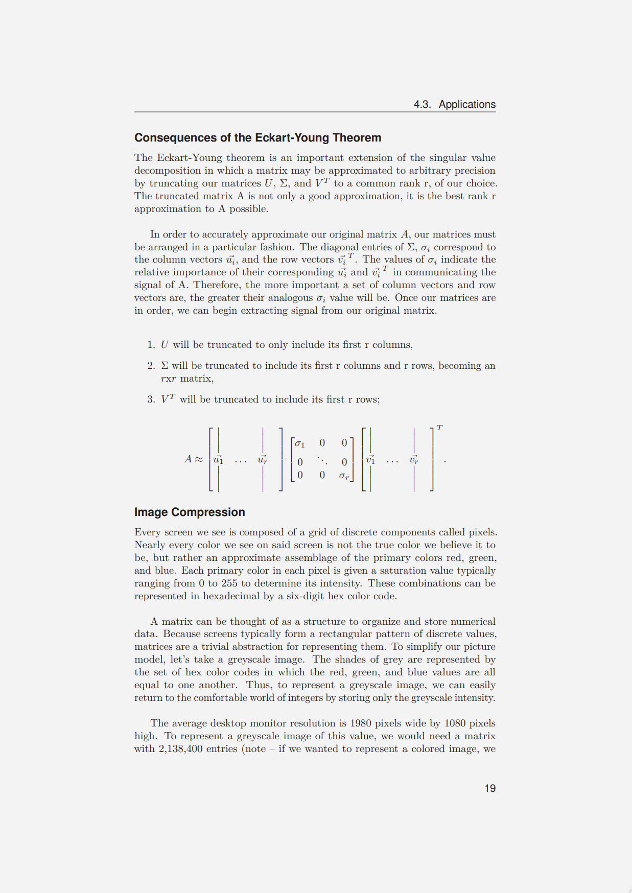
Consequences of the Eckart-Young Theorem. The Eckart-Young theorem is an important extension of the singular value decomposition in which a matrix may be approximated to arbitrary precision by truncating our matrices $U$, $\Sigma$, and $V^T$ to a common rank $r$, of our choice. The truncated matrix $A$ is not only a good approximation, it is the best rank $r$ approximation to $A$ possible.

In order to accurately approximate our original matrix $A$, our matrices must be arranged in a particular fashion. The diagonal entries of $\Sigma$, $\sigma_i$ correspond to the column vectors $\vec{u_i}$, and the row vectors $\vec{v_i}^T$. The values of $\sigma_i$ indicate the relative importance of their corresponding $\vec{u_i}$ and $\vec{v_i}^T$ in communicating the signal of $A$. Therefore, the more important a set of column vectors and row vectors are, the greater their analogous $\sigma_i$ value will be. Once our matrices are in order, we can begin extracting signal from our original matrix:

1. $U$ will be truncated to only include its first $r$ columns,
2. $\Sigma$ will be truncated to include its first $r$ columns and $r$ rows, becoming an $r \times r$ matrix,
3. $V^T$ will be truncated to include its first $r$ rows;

Image Compression

Since images can be represented as matrices of pixel intensities, SVD provides a natural compression scheme. A 1920x1080 greyscale image requires over 2 million entries. By keeping only the top-$r$ singular values, we can dramatically reduce storage while preserving visual fidelity.

SVD-based image compression applied to the Georgia Highlands College campus, showing approximations at ranks 1, 5, 30, 65, 80, and 100.

Collaborative Filtering

Netflix, Amazon, and other recommender systems use SVD-based techniques to extract patterns from user-item interaction matrices. By decomposing a sparse ratings matrix, collaborative filtering can predict what a user might enjoy based on the preferences of similar users.

Latent Semantic Indexing

LSI uses the truncated SVD to process natural language, enabling computers to see past synonymy (different words, same meaning) and polysemy (one word, multiple meanings) by analyzing word usage structure across documents.

Why This Matters

These four decompositions form the computational backbone of modern scientific computing and machine learning:

• LU is the workhorse behind solving systems of linear equations
• Eigendecomposition powers PCA, spectral clustering, and dynamical systems analysis
• Jordan form gives us efficient matrix exponentiation for recurrences and differential equations
• SVD underlies everything from image compression to recommendation engines to NLP

Understanding them at the matrix level — not just as API calls — is what separates engineers who can debug numerical instability from those who can’t.

This paper was written as an extracurricular honors project at Georgia Highlands College. Thanks to Dr. Paul J. Kapitza for supervising the project and for demonstrating that spending time on fundamentals leads to substantial revelations.

Download the full paper (PDF)